Environment for creative processing of text and numerical data |

|
Environment for creative processing of text and numerical data |
|
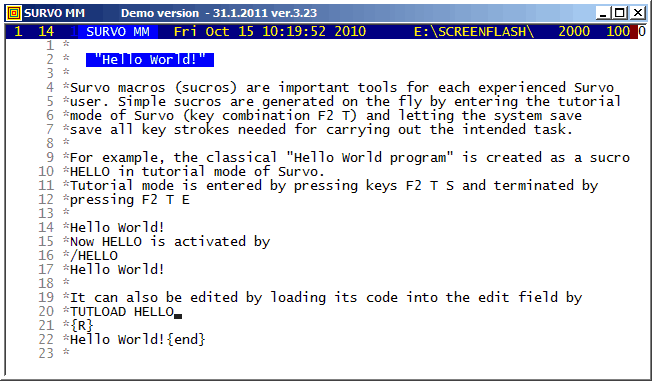
Example #1 (Start the demo by clicking the picture!)
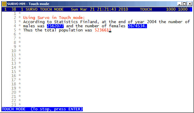
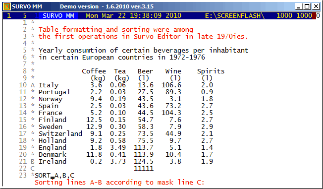
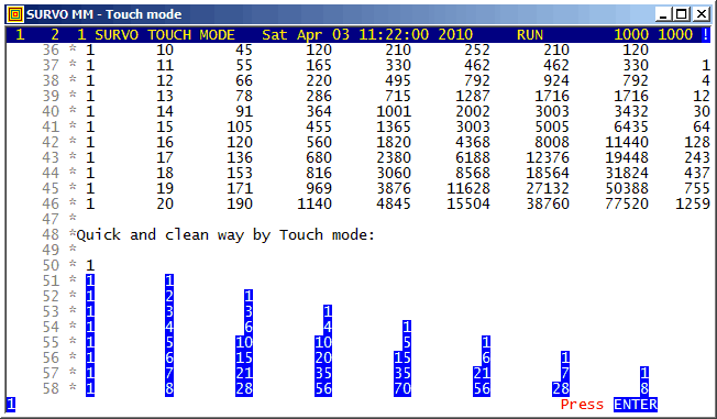
Touch mode is one of the smart calculation modes in Survo.
The function key F3 is the TOUCH key for entering the Touch mode of the Survo editor.
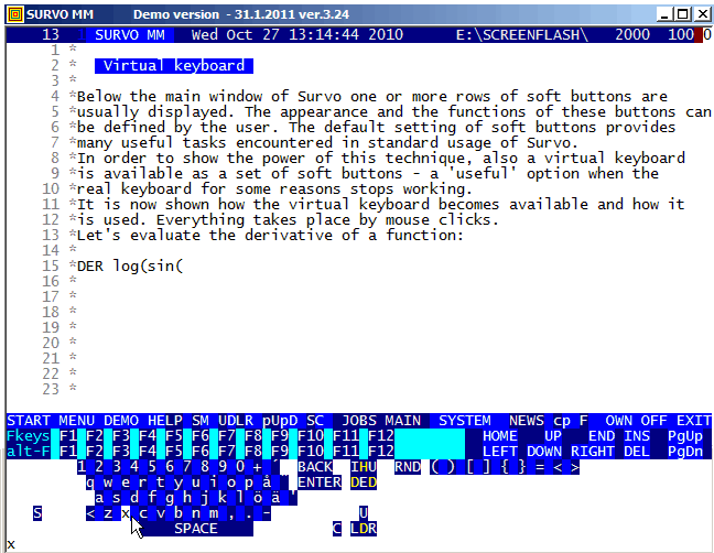
Example #2 (Start the demo by clicking the picture!)
Survo Graphics windows typically do not overlay the Survo main window. However, in these GIF-animations the graphs are placed on the main window.
Example #4 (Start the demo by clicking the picture!)
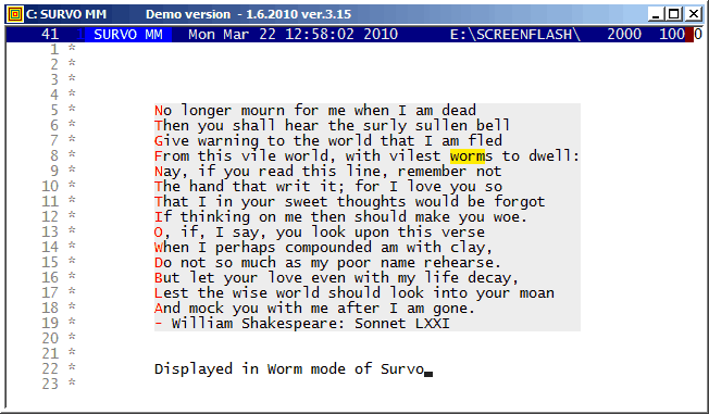
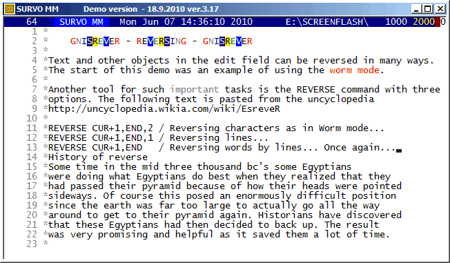
When some computer specialists claimed that Survo is able for 'simple text editing only', "Worm mode" was created in 1994 for demonstrating that they were wrong :)
Example #5 (Start the demo by clicking the picture!)
This demo in YouTube
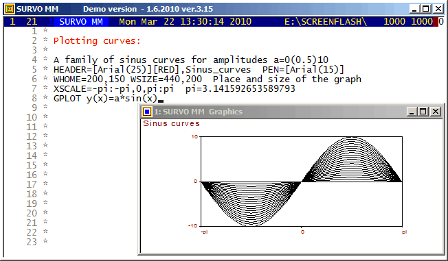
As a technical detail, it also shown how the graph of the sample is positioned in the display.
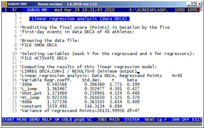
Screen graphics (created by GPLOT commands of Survo) are displayed by default in separate windows typically outside the Survo main window.
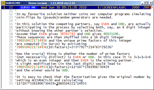
Example #6 (Start the demo by clicking the picture!)
This demo in YouTube
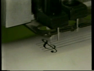
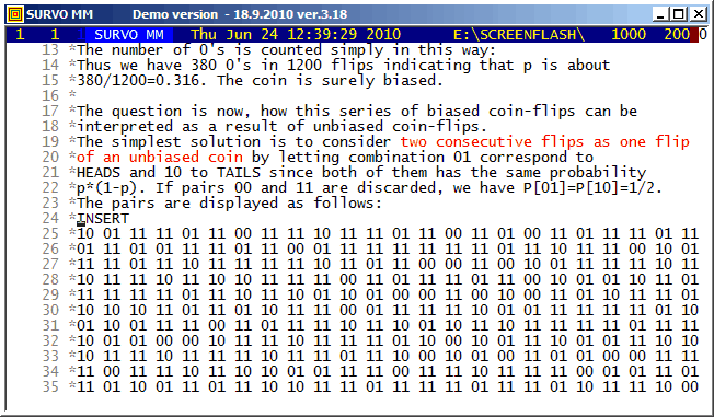
The editorial approach was originally created for a musical application.
See
Example of the first version of Survo Editor.
Example #7 (Start the demo by clicking the picture!)
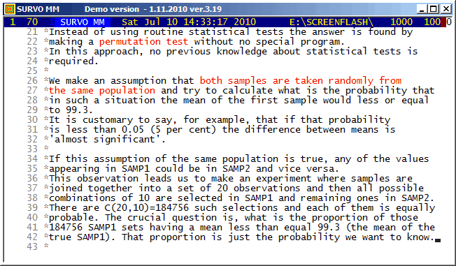
Survo Graphics windows typically do not overlay the Survo main window. However, in these GIF-animations the graphs are placed on the main window.
Example #8 (Start the demo by clicking the picture!)
This demo in YouTube
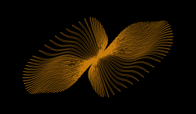
A closed curve defined by a plotting scheme
HEADER= FRAME=0 MODE=1024       XDIV=0,1,0 YDIV=0,1,0
T=0,2*pi,pi/4000 pi=3.14159265 XSCALE=-3.0,3.0 YSCALE=-1.5,1.5
R=cos(78*T)+cos(80*T) A=R*cos(T) B=R*sin(T)
s=0.8 u=0.06 LINETYPE=[color(0.1,0.3,1,0.2)]  COLORS=[/BLACK]
SLOW=400
GPLOT X(T)=A+s*B+u*sin(5*B),Y(T)=B+u*sin(5*A)
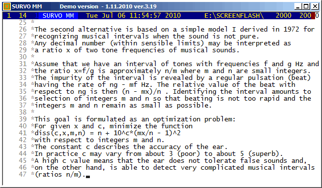
Example #9 (Start the demo by clicking the picture!)
This demo in YouTube
In fact, all these GIF animations were originally made as such tutorials by letting the ScreenFlash program to 'watch' them and save as Flash movies. These movies were then converted to GIF animations by the same program.
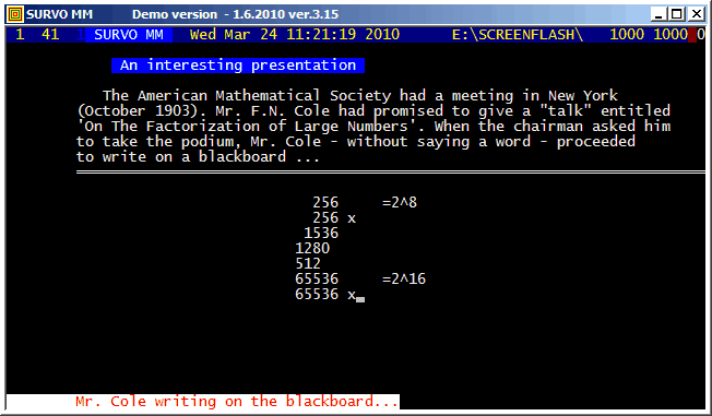
This example was also present in 1990 in a school version of Survo. The aim here was to point out how diligent people in old times - without computers and calculators - were ready and able to do very demanding numerical computing.
The arithmetical calculations presented here were carried out by a family of arithmetical sucros (<Survo>\OPETUS\AR) made just for this presentation.
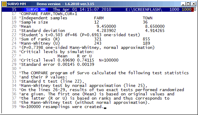
A related demo: Prime factors of numbers m^n-1
Example #10 (Start the demo by clicking the picture!)
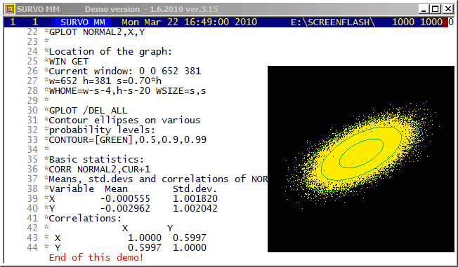
This demo in YouTube
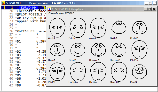
Survo offers several means for illustration of multivariate statistical
data.
One of them is
Chernoff's faces.
The original numerical data was given
here
(almost 20 years before Chernoff invented his faces).
Example #12 (Start the demo by clicking the picture!)
This demo in YouTube
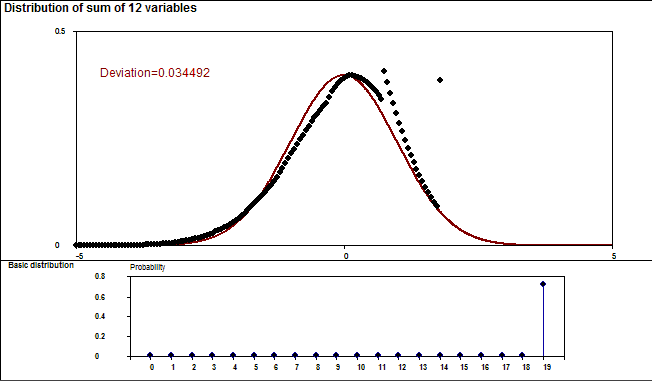
This demo illustrates the power of the Central limit theorem of probability and statistics.
In each stage it is shown graphically how close the standardized sum distribution is to the normal distribution. The gap between the sum and the normal distribution is also given numerically as a deviation corresponding to the standard Kolmogorov-Smirnov test statistics.
Two examples are shown. The first one tells how the binomial distribution tends quickly to normal distribution. The second example (due to a very heavy tail on the right) has more dramatic features but eventually normalization is its inevitable destiny, too.
Example #13 (Start the demo by clicking the picture!)
This demo in YouTube
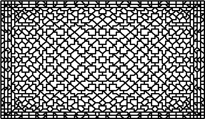
The graph here is slightly simplified, due to a limited resolution on the screen but given as a stepwise presentation revealing the complete symmetry finally at the last steps.
The basis of the graph is a Lissajous curve getting a more surprising appearance by "rounding" the function values to integers.
The entire setup in a Survo edit field for making the graph is
GPLOT X(T)=int(M*sin(N*T)+0.5),
      Y(T)=int(N*cos(M*T)+0.5)
M=29 N=19 T=[line_width(4)],0,2*pi,pi/3100 pi=3.14159
HEADER= FRAME=0 XSCALE=-M,M YSCALE=-N,N
XDIV=0,1,0 YDIV=0,1,0
MODE=652,381 WSIZE=652,381 WHOME=0,0 WSTYLE=0
SLOW=300 Slowing the speed by drawing each line segment 300 times
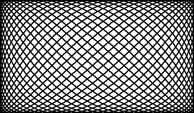
The corresponding Lissajous curve without "rounding" by int():
Example #14 (Start the demo by clicking the picture!)
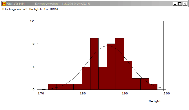
Plotting the histogram of variable Height in data DECA (N=48)
and fitting to normal distribution:
GHISTO DECA,Height,CUR+2 / Height=170.5(2)200.5 FIT=Normal
Frequency distribution of Height in DECA: N=48
Class midpoint f % Sum % e e f X^2
171.5 0 0.0 0 0.0 0.1
173.5 1 2.1 1 2.1 0.2
175.5 1 2.1 2 4.2 0.6
177.5 1 2.1 3 6.3 1.4
179.5 1 2.1 4 8.3 2.7 5.1 4 0.2
181.5 4 8.3 8 16.7 4.4
183.5 9 18.8 17 35.4 6.2 10.6 13 0.5
185.5 4 8.3 21 43.8 7.4 7.4 4 1.6
187.5 8 16.7 29 60.4 7.5 7.5 8 0.0
189.5 9 18.8 38 79.2 6.6 6.6 9 0.9
191.5 5 10.4 43 89.6 4.9
193.5 2 4.2 45 93.8 3.1
195.5 2 4.2 47 97.9 1.7
197.5 1 2.1 48 100.0 0.8
199.5 0 0.0 48 100.0 0.3 10.8 10 0.1
Mean=186.7500 Std.dev.=4.993746
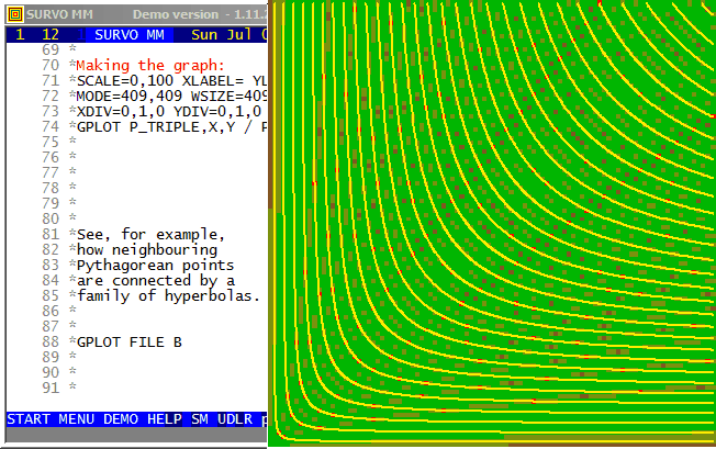
Fitted by NORMAL(186.75,24.9375) distribution
Chi-square=3.297 df=3 P=0.3480
No significant departure from normal distribution!
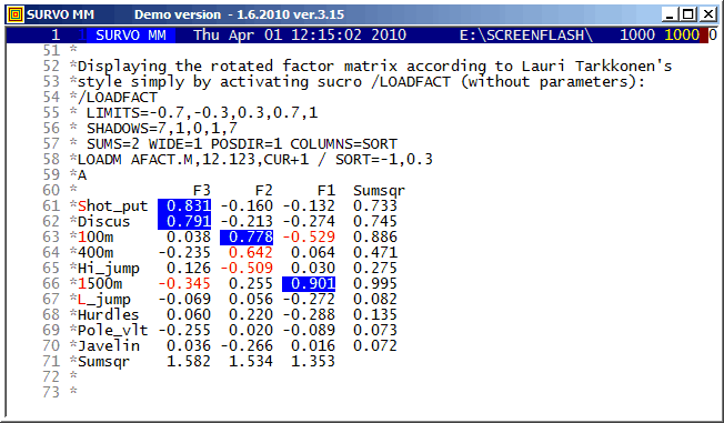
There are many options in Survo for factor analysis and related topics.
This is a straightforward example of the classical approach.
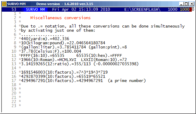
Numerical conversions in the editorial mode were included in 1988.
This demo is created by Kimmo Vehkalahti.
It is a good example of co-operation between Editorial computing and Survo data file operations.
This demo in YouTube
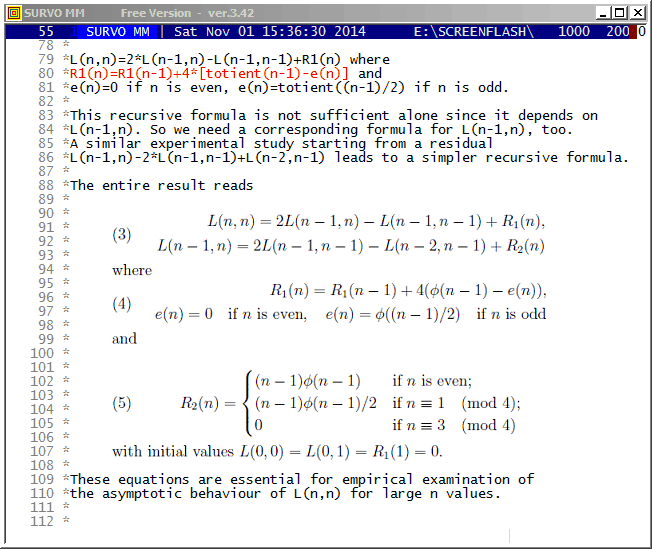
The formulas behind the computational setup
L(N)|=if(N<2)then(0)else(2*L1(N)-L(N-1)+R1(N))
L1(N)|=if(N<3)then(1)else(2*L(N-1)-L1(N-1)+R2(N)) R1(N):=4*S(N)
S(N):=for(I=2)to(N)sum(totient(I-1)-e(I))
e(N):=if(mod(N,2)=0)then(0)else(totient((N-1)/2))
R2(N):=if(mod(N,2)=0)then((N-1)*totient(N-1))else(R21(N))
R21(N):=if(mod(N,4)=1)then((N-1)*totient(N-1)/2)else(0)
Another formula in Sloane's Encyclopedia of Integer Sequences has been presented earlier but it is much slower in computations.
Before finding the fast recursive formulas, I could make a conjecture
that an accurate asymptotic expression for L(n) is
L(n)=[3/(2*pi)*n^2]^2+O(n^2.5)
based on calculations for values n<=15000 by the slow formula as told in my document on pages 8-9.
Later (by using the fast formulas) I have computed the L(N) values for all N values to 10^11 by Mathematica code (on page 27) controlled directly from Survo. The graph indicates that the accuracy of the asymptotic expression really seems to be of order O(n^2.5) and this conjecture has been validated in a paper by Ernvall-Hytönen, Matomäki, Haukkanen, and Merikoski provided that the Riemann hypothesis is true. In the same paper also my other empirical findings have been proved.
Finding recursive formula for number of grid lines
*TUTSAVE BIN-CONV
/ /BIN-CONV number,n
* converts a positive decimal number <1 into binary form with n bits.
/ def Wx=W1 Wacc=W2 Wn=W3 Wint=W4
/
*{init}{tempo -1}{Wn=0}{Wint=0.}{R}{erase}
+ A: {Wx=2*Wx}{ref}{line end}{print Wint}{R}
*{erase}int({print Wx})={act}{l} {save word Wint}{Wx=Wx-Wint}
*{Wn=Wn+1}
- if Wn < Wacc then goto A
*{line start}{erase}
+ E: {tempo +1}{end}
*
*
*TUTSAVE BIN-SUB
/  /BIN-SUB makes the difference of two binary numbers,
/  either integers or fractions in (0,1) according to following setup:
/
/           ..  ....   ....  (borrowed bits appearing during calculation)
/           1001110000110010 A
/  /BIN-SUB 0010010010100111 B  (activate at the last bit)
/           0111011110001011 A-B
/
*{tempo -1}
+ A: {ref set 1}{save char W1}
- if W1 '=' {sp} then goto E
- if W1 '=' . then goto B
- if W1 '=' 0 then goto C
/ W1=1
*{u}{save char W2}
- if W2 '=' 1 then goto D1
*{u}{save char W2}{d}
- if W2 '=' . then goto D2
/
+ F: {l}{u}.{l}{d}{save char W2}
- if W2 '=' 0 then goto F
*{ref jump 1}{W3=1}{goto S}
+ D1: {u}{save char W2}{d}
- if W2 '=' . then goto D3
*{d}{W3=0}{goto S}
+ D3: {goto F}
+ D2: {d}{W3=0}{goto S}
/
+ C: {u}{save char W2}
- if W2 = 1 then goto C1
*{u}{save char W2}{d}
- if W2 '=' . then goto C2
*{d}{W3=0}{goto S}
+ C2: {d2}1{ref jump 1}{l}{goto A}
+ C1: {u}{save char W2}{d}
- if W2 '=' . then goto C3
*{d}{W3=1}{goto S}
+ C3: {d}{W3=0}{goto S}
+ B: {W3=.}
+ S: {d}{print W3}{ref jump 1}{l}{goto A}
+ E: {tempo +1}{end}
This demo in YouTube
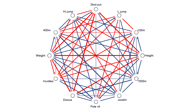
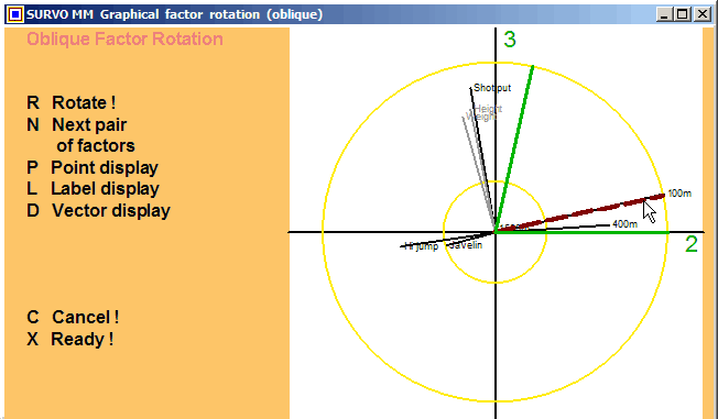
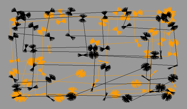
It is not possible to make this kind of graphs quite automatically since there are so many options. However, a ready-made template corresponding to this example exists for Survo users. It is easy to modify this template for at least up to correlation matrices with 30 variables and get a good general view on the relations at hand.
To gain enough accuracy, this arrow or vector diagram is drawn as a PostScript picture. The final picture is obtained by combining two graphs using the EPS JOIN command of Survo for PostScript files generated by Survo PLOT commands. The final display here is dramatically slowed down by a SLOW=3000 specification when making the arrow diagram.
This demo in YouTube
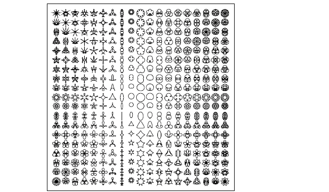
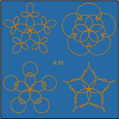
The graph illustrates a fact how little information is needed for creating various forms starting from a simple circle (ovum) at the center. The plotting scheme
XDIV=0,1,0 YDIV=0,1,0 SIZE=1180,1180 HEADER= FRAME=3 HOME=300,500
A=-8,10,1        B=-8,10,1        T=0,2*pi,pi/30 pi=3.14159265
XSCALE=-9,11     YSCALE=-9,11     DEVICE=PS,SPECIES.PS

PLOT X(T)=A+0.225*SIN(T)+0.139*SIN(A*T)+0.086*SIN(B*T),
     Y(T)=B+0.225*COS(T)+0.139*COS(A*T)+0.086*COS(B*T)

/GS-PDF SPECIES.PS
A more accurate version (tenfold size and step length pi/300) is made as follows:
*XDIV=0,1,0 YDIV=0,1,0 SIZE=11800,11800 HEADER= FRAME=3 HOME=0,0
*A=-8,10,1        B=-8,10,1        T=[line_width(0.96)],0,2*pi,pi/300
*pi=3.141592653589793
*XSCALE=-9,11     YSCALE=-9,11     DEVICE=PS,SPECIES10.PS
*
*PLOT X(T)=A+0.225*SIN(T)+0.139*SIN(A*T)+0.086*SIN(B*T),
*     Y(T)=B+0.225*COS(T)+0.139*COS(A*T)+0.086*COS(B*T)
*
*.....................................................................
*PRINT CUR+1,E TO K.PS / Reduction to original size
% 1240
- [left_margin(1)]
- picture species10.ps,*,*,0.1,0.1
E
I had done same things one year before for the Wang PC by using interpretative Basic. When I heard some programming experts in Finland to say that "Basic spoils your brain!":) I wanted to test my brain when getting a chance to start learning C by selecting these rather demanding targets as my first examples in C programming.
Usually I wrote already then all my programs at the computer without pen and paper but all this happened during Summer 1985 during my summer vacation in Central Finland where I had no access to any computer. So I wrote these programs by hand and got the first chance to test them only after returning home in August and by starting using my brand new IBM PC (AT model) and the new Microsoft C compiler.
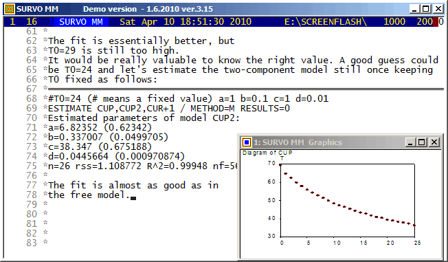
This tiny example tells how ESTIMATE is used in calculating parameters and related statistics of a nonlinear regression model. The predecessor of ESTIMATE (on Wang PC in 1984) was probably one of the first statistical programs able to evaluate symbolic derivatives automatically and see (by studying derivatives of the second degree of the model function) whether they all are zero or not and thus determine if the model is linear with respect to parameters to be estimated or not. Then the program could decide what kind of numerical algorithm to select.
The the first model in this example was
MODEL CUP1 / Exponential decay
T=T0+a*exp(-b*t)
ESTIMATE is able to distinguish what are the parameters to be estimated (a,b) since it detects that T and t are variables in the data set CUP.
I made the original Finnish version of this demo in 1990 in connection with a limited SURVOS version intended for use in Finnish schools.

SIZE=681,381 XDIV=0,1,0 YDIV=0,1,0 MODE=681,381
SCALE=0,7 FRAME=0 SLOW=100
t=0,50,1 n=0,35,1 r=-1.0,-0.1,0.1
GPLOT X(t)=int(n/6)+1+r*cos((-7*r+n)*t),
      Y(t)=n+1-6*int(n/6)+r*sin((-7*r+n)*t)
COLORS=[/BLACK]
COLOR_CHANGE=n-10*r,16
The COLOR_CHANGE specification takes care of selecting one of 16
colors according to value mod(n-10*r,16).
SLOW=100 makes the output 100 times slower than normally.
This demo in YouTube
I encountered this problem when making the first computer program
in 1962 for Cosine rotation in factor analysis.
This rotation technique was devised and applied as a hand calculation
and graphical procedure by by Yrjö Ahmavaara and Touko Markkanen in the
1950ies.
As far as I know, before 1962 no analytical approach to the problem of
selecting the 'factor variables' had been presented.
In the cosine rotation program the target is to select the factor
variables as the maximally orthogonal subset of variables by a determinant
criterion. That principle is demonstrated in this example.
This demo in YouTube
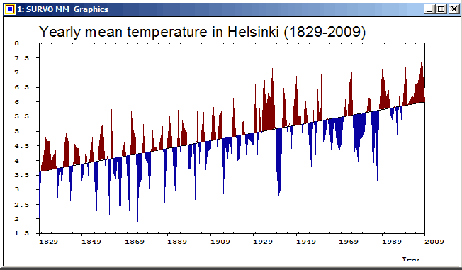
This graph of a time series was created by the Survo plotting scheme:
YLABEL=[Arial(25)],Yearly_mean_temperature_in_Helsinki_(1829-2009)
GPLOT HEL_MEAN,Year,Temp / SIZE=652,381 YDIV=50,291,40
XSCALE=1829(20)2009 YSCALE=1.5(0.5)8  TICK=5,1 TICK2=5,1
LINE=[WHITE],1 TREND=[BLACK],0 PEN=[BLACK]
FILL=[RED],1,1,181,Trend,1 FILL-=[BLUE]
XDIV=50,539,50 HEADER=   WHOME=0,0 WSIZE=652-5,381-25
This demo in YouTube
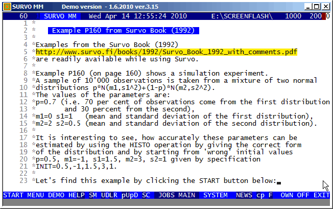
Here is the entire setup in the edit field for making this experiment:
FILE CREATE SIMUDATA,4,1,64,7,10000
  Sample (N=10000) from a mixture of two normal distributions
FIELDS:
1 N 4 X
END

VAR X TO SIMUDATA
  X=if(rnd(1)<0.7)then(X1)else(X2)
  X1=probit(rnd(1))
  X2=0.5*probit(rnd(1))+2
.......................................................................

DENSITY MIXNORM(p,m1,s1,m2,s2)
y(x)=c*(p/s1*exp(-0.5*((x-m1)/s1)^2)+(1-p)/s2*exp(-0.5*((x-m2)/s2)^2))
     c=0.39894226
GHISTO SIMUDATA,X,22
X=-10(0.2)10 XSCALE=-10(2)10 YSCALE=0(100)600
FIT=MIXNORM INIT=0.5,0.5,1.5,2.5,0.7

HISTO: Estimated parameters of MIXNORM:
p=0.7044 (0.0123)
m1=0.0088 (0.0290)
s1=1.0136 (0.0185)
m2=2.0186 (0.0200)
s2=0.5200 (0.0139)
...
This technique is available in SURVO MM versions 3.16+.
This demo in YouTube
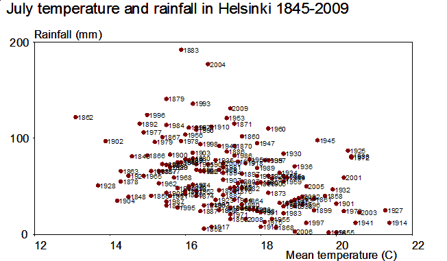
Although there is much confusion in labels in the middle of the graph, the exceptional and thus the most interesting years can be clearly detected. The first versions of this graph were made in late 1970ies by using SURVO 76.
In Survo a special program called by a GEOM command is available for making such constructions in conjunction with some other Survo functions.
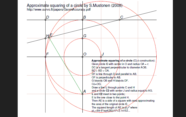
Here a construction for approximate circle squaring is presented.
It is based on a random search in a square grid as explained in my paper
Statistical accuracy of geometric constructions (2008)
on pages 35-37.
This construction is described in an edit field as follows:
*/GEOM
*GEOM CUR+1,E
*CL4
*O=point(2,2)
*A=point(2,0)
*_C1=circle(O,2)
*LX4=line(A,O)
*B=cross_cl(C1,LX4,2,4)
*c2=circle(B,*2)
*LY4=perpendicular(LX4,*B)
*C=cross_cl(C2,LY4,4,4)
*D=cross_cl(C2,LY4,0,4)
*LY2=perpendicular(LX4,O)
*LX2=perpendicular(LY4,*D)
*F=cross(LX2,LY2)
*G=midpoint(B,O,LX4)
*H=midpoint(D,F,LX2)
*C3=circle_p(O,G)
*J=cross_cl(C3,LY2,3,2)
*eag=edge(A,G)
*C4=circle(J,EAG)
*L=line(H,C)
*E=cross_cl(C4,L,0,3)
*Edge=edge(A,E)
*save edge(Edge)
E
GEOM is typically called by a sucro /GEOM which creates suitable Survo data files for various geometric objects appearing in the construction. Thus /GEOM also calls GEOM for making the construction so that points are saved in _POINTS.SVO, lines in _LINES.SVO, circles in _CIRCLES.SVO, and edges in _EDGES.SVO.
The construction can then be displayed by using various forms of the Survo operation PLOT. An ready-made template as a SURVO edit field is available so that the entire construction is saved as a PostScript file.
Everyone who has experience of making geometric constructions in practice knows how much attention must be paid to a careful placement of the compass and the straightedge in each step of the construction in order to achieve as accurate results as possible.
In my paper, the accuracy of these placements is described by a simple statistical model and the accuracy of the entire construction is estimated on this basis. Then it is natural to consider the accuracy of the construction as a measure of its complexity. This measure is expected to give better possibilities for comparing complexities of constructions than the characteristics of Lemoine's geometrography. My approach is mainly computational. Although the error distribution of placements is defined precisely, the error distributions related to entire constructions are so complicated that the only way is to use Monte Carlo simulation for estimating essential statistics.
When considering the accuracy of this approximate circle squaring construction, the nominal accuracy (pi-3.14152=0.00007) is not a sufficient measure since it can be attained only when there are no errors in construction steps.
For example, the relative root mean squared error (defined on page 24 and computed on page 37 of my paper) of this construction is 2.125 while, for example, that of Kochanski when extended to approximate construction of sqrt(pi)r (the side of the square) is 2.908, although the nominal accuracy of the latter is 0.00006 and thus slightly better.
This demo in YouTube
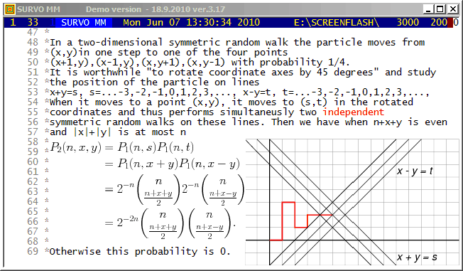
The background of this presentation is William Feller's An Introduction to Probability Theory and Its Applications, Vol.I (Second Edition 1957) Ch. XIV.7 "Random Walks in the plane and space".
As a student of mathematics and statistics I wrote an essay about this topic in 1959 after inventing a simpler formula for the transition probability (of moving from the origin to the point (x,y) in n steps) compared to that given as a double integral expression by Feller.
I sent a letter about my findings to Feller and got immediately a friendly answer from him where he promised to use my result "if any" in the forthcoming edition of his book. However, to my disappointment, in next editions nothing had been changed in this respect.

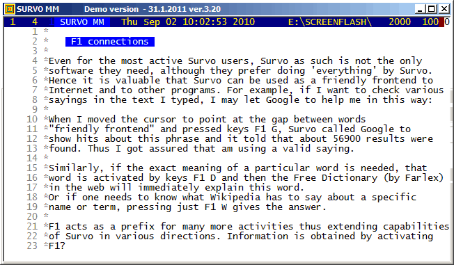
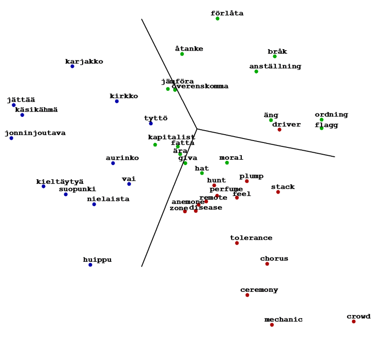
F1 J is an extended alternative for F2 J for completing phrases found elsewhere in the current edit field. As in this example, a list containing 'all possible phrases' may be loaded to the end of the edit field. This list then serves as a source of information during writing process by giving synonyms, technical terms etc.
It is easy to create such lists on different topics by pasting them from websites, for example. The list used in this example originates from Birds of Sweden.
This demo in YouTube
This feature has been available already in SURVO 76.
The traditional graphical rotation is described e.g. in
Ledyard Tucker and Robert MacCallum:
Exploratory Factor Analysis,
Chapter 10.
The principles of Cosine rotation and Transformation analysis were
introduced in Yrjö Ahmavaara's dissertation
Transformation Analysis of Factorial Data, Helsinki Ann.
Acad. Sci. Fenn., B 88, 2, 1954.
The current algorithm for Cosine rotation was created in 1961 and
described in
Matrix computations in Survo
This demo in YouTube
A comprehensive documentation is given in my paper
Visualization and characterization of Pythagorean triples.
Interactive 'graphical' identifying of Pythagorean triples is available
as a sucro /P_TRIPLE.
The original data of 1200 flips with a biased coin (p=1/3) was generated by Survo as follows:
FILE CREATE COIN,1,1
FIELDS:
1 N 1 X
END

FILE INIT COIN,1200

p=1/3
MATRIX P ///
0 p
1 1-p

MAT SAVE P

RND=URAND(20106)
TRANSFORM COIN BY #DISTR(P)
MAT SAVE DATA COIN AS COIN2
MAT COIN3=VEC(COIN2,20)      / *COIN3~VEC(COIN2) 20*60

MAT LOAD COIN3,##,CUR+1
MATRIX COIN3
VEC(COIN2)
///       1  2  3  4  5  6  7  8  9 10 11 12 13 14 15 16 17 ...
  1       1  0  0  1  1  1  1  1  0  1  1  1  0  0  1  1  1 ...
  2       0  1  1  1  0  1  0  1  1  1  1  1  0  1  1  1  0 ...
  3       1  1  1  1  0  1  1  1  1  0  1  1  1  1  1  1  1 ...
  4       1  0  1  1  1  1  1  0  1  1  1  0  1  0  1  1  1 ...
  5       1  1  1  1  1  1  1  1  0  1  1  1  1  0  1  1  1 ...
  .       .  .  .  .  .  .  .  .  .  .  .  .  .  .  .  .  . ...
To give credence to the fact that the number of prime factors is even or odd with probablity 1/2, I took a random sample of 10 million integers with 16 digits by the following Mathematica code
a=10^15
SeedRandom[1];
t1=TimeUsed[];
tab:=Table[PrimeOmega[RandomInteger[{a,a+8999999999999999}]],{n,1,10^7}];
Export["Sample.txt",tab,"Table"]
TimeUsed[]-t1
Omega      f     %      *=65536 obs.
  1   277575   2.8 ****
  2  1053208  10.5 ****************
  3  1860960  18.6 ****************************
  4  2105565  21.1 ********************************
  5  1783889  17.8 ***************************
  6  1245149  12.5 ******************
  7   765283   7.7 ***********
  8   433642   4.3 ******
  9   232340   2.3 ***
 10   120919   1.2 *
 11    60947   0.6 :
 12    30650   0.3 :
 13    15225   0.2 :
 14     7482   0.1 :
 15     3655   0.0 :
 16     1814   0.0 :
 17      876   0.0 :
 18      408   0.0 :
 19      217   0.0 :
 20      102   0.0 :
 21       49   0.0 :
 22       22   0.0 :
 23       15   0.0 :
 24        3   0.0 :
 25        2   0.0 :
 27        1   0.0 :
 28        1   0.0 :
 29        1   0.0 :
In number theory the function lambda(n)=(-1)^Omega(n) getting "randomly" values -1 and +1 is known as Liouville function and it completely corresponds to "Omega coin tossing". The sums of lambda(n) has been studied experimentally in Sign changes in sums of the Liouville function by Borwein, Ferguson, and Mossinghoff (2010).
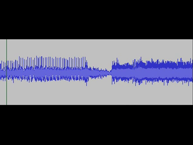
The VAR and PLAY commands of Survo give an opportunity to create and play sound files (in WAV format). For example, the neutral third and pure intervals close to can be listened as follows:
s(X):=sin(X*ORDER)

f1=11/9 1.2222222222222...          Interval_11_9
f2=sqrt(5/4*6/5) 1.2247448713916... Neutral_third
f3=5/4 1.25                         Major_third
f=0.2 'basic frequency'

FILE MAKE Test,1,24000,X,2            / creates data file Test.
VAR X=10000*(s(f)+s(f*f1)) TO Test    / computes the wave form
PLAY DATA Test,X / WAV=Interval_11_9  / converts the wave form into WAV
VAR X=10000*(s(f)+s(f*f2)) TO Test
PLAY DATA Test,X / WAV=Neutral_third
VAR X=10000*(s(f)+s(f3*f)) TO Test
PLAY DATA Test,X / WAV=Major_third

PLAY SOUNDS                           / plays sound files created
Interval_11_9
Neutral_third
Major_third

Slightly off the topic:
The neutral third sqrt(3/2) is recognized correctly from its
approximate value 1.2247448713916 by the INTREL command
INTREL 1.2247448713916 / giving
X=1.2247448713916 is a root of 2*X^2-3=0
This demo in YouTube
In the plotting scheme the jumps are triggered by int() functions in X(t) and Y(t) expressions.
HEADER=  HOME=0,0 WHOME=0,0 WSIZE=652,381 WSTYLE=0 MODE=652,381
XSCALE=-14,14 YSCALE=-10,10 FRAME=3
SIZE=652,381 XDIV=0,1,0 YDIV=0,1,0
a=53 t=0,50*pi,pi/150 pi=3.14159
GPLOT X(t)=12*sin(int(0.35*t))+0.8*sin(a*t)*sin(t)+0*A,
      Y(t)=8*sin(int(0.3*t))+0.8*sin(a*t)*cos(t)
A=0(1)4
PALETTE=BGY3 COLORS=[background(8)] COLOR_CHANGE=A,3
SLOW=100 slowing down the plotting speed
This is an abbreviated version of a Finnish teaching program made in
1998.
The COMB operation and the Survo matrix interpreter are the key components in this experiment. Also a few other special features of Survo are applied.
This demo in YouTube
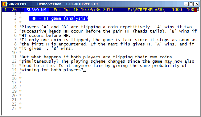
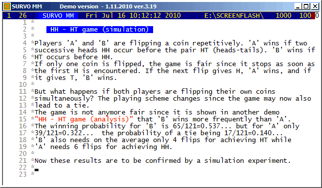
This example is continued by a simulation experiment HH - HT game (simulation)
This demo in YouTube
This demo in YouTube (created in 2010)
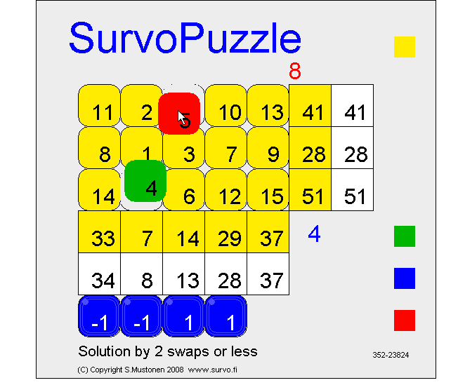
I presented
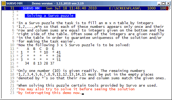
Survo Puzzle
in 2006. More information is available on the
home page.
Survo supports solving of these puzzles in many ways. Besides the COMB operation also Editorial computing and Touch mode are useful tools. The editorial interface of Survo is also suitable for general book-keeping during the solving process.
This demo in YouTube
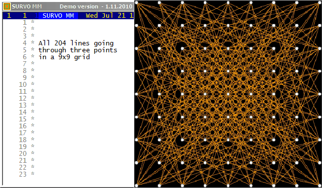
This is an illustration related to my paper
On lines through a given number of points in a rectangular grid of points.
On the cover page of that paper this picture of
all L(16,4)=548 lines connecting exactly four points in a 16x16 grid
is presented:
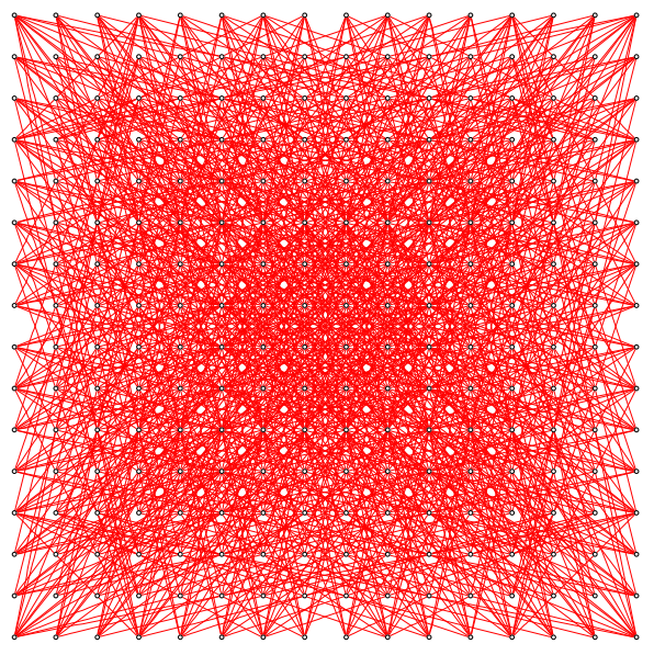
Although efficient computing of numbers L(n,j), i.e. # of lines going through j points in and nxn grid of points, is not trivial, making a list of these lines is still more demanding task for large n values. However, such a list for small n is easy to generate by brute force on current computers. Thus the Survo program module GRIDP simply starts from all pairs of points in the grid and sorts out the required lines.
This demo in YouTube
If this puzzle is given as an open Survo puzzle without any fixed numbers in the form
    A  B  C  D  E
 1  *  *  *  *  * 41
 2  *  *  *  *  * 28
 3  *  *  *  *  * 51
   34  8 13 28 37
it has also another solution which is obtained by three swaps.
Try to find that solution by going to
https://www.survo.fi/swap/puzzles
and click the game board and type #352-23824 ENTER
If your browser does not support Java, a corresponding Javascript version is available.
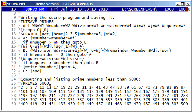
The prime numbers are found by using a variation of the 'trial division'
method:
After numbers 2, 3, and 5 are listed, both n values (Wnumber in PRIMES) and m values (Wfactor) are selected so that they are not divisible by 2 or 3.
A sucro program cannot be efficient in purely numerical problems
since all objects processed by a sucro are presented as strings of
characters. The 'values' of variables are saved in a 'sucro memory'
which is simply a string.
For example, at the end of the current application
this string is
In typical applications of sucros, like teaching programs and demos (like these GIF animations) and combining several Survo operations, this feature is unimportant. Although Survo program modules are written in C, many system routines are sucros.
A general description of the sucro language is given in User Guide (1992) chapter 12 (pages 399 - 443).
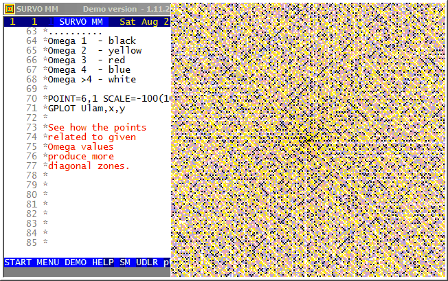
Background information about the Ulam spiral in Wikipedia, for example.
When making the spiral the main task is to map values of n to x,y
coordinates.
I derived the formulas
x(n)=x(n-1)+sin(mod(int(sqrt(4*(n-2)+1)),4)*pi/2)
y(n)=y(n-1)-cos(mod(int(sqrt(4*(n-2)+1)),4)*pi/2)
by observing that the turning points of the spiral may be described in
this way
           12 11 11 11 11 11 11
           12  8  7  7  7  7 10  .
           12  8  4  3  3  6 10  .
           12  8  4  1  2  6 10 14
           12  8  5  5  5  6 10 14
           12  9  9  9  9  9 10 14
           13 13 13 13 13 13 13 14
1,2,3,3,4,4,5,5,5,6,6,6,7,7,7,7,8,8,8,8,9,9,9,9,9,...
with a general term a(n)=int(sqrt(4n+1)), n=0,1,2,...
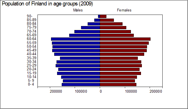
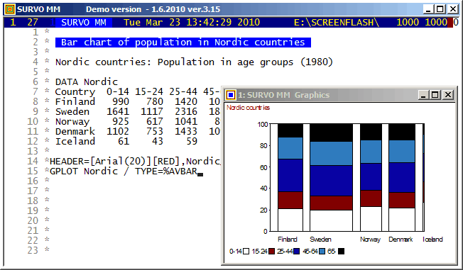
The age pyramid (TYPE=PYRAMID) is one of types of bar charts in Survo.
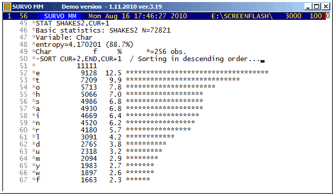
Shakespeare's 154 Sonnets were imported from
http://www.shakespeares-sonnets.com.
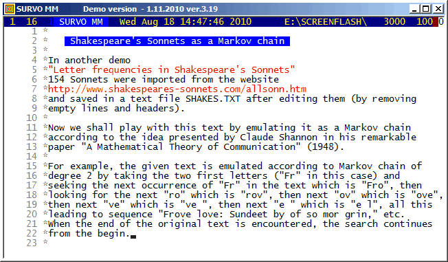
The same textual data is studied in demos
Shakespeare's Sonnets as a Markov chain and
The most common words in Shakespeare's Sonnets.
The letter frequencies in Shakespeare's Sonnets counted in this demo seem to deviate significantly from current English at least for some common letters like a,c,h,t as one can see in the following table.
Letter  Sonnets English Difference
          %       %
a       6.8     8.2    -1.4
b       1.7     1.5     0.2
c       1.8     2.8    -1.0
d       3.8     4.3    -0.5
e      12.5    12.7    -0.2
f       2.3     2.2     0.1
g       1.9     2.0    -0.1
h       7.0     6.1     0.9
i       6.4     7.0    -0.6
j       0.1     0.2    -0.1
k       0.8     0.8     0.0
l       4.2     4.0     0.2
m       2.9     2.4     0.5
n       6.2     6.7    -0.5
o       7.8     7.5     0.3
p       1.4     1.9    -0.5
q       0.1     0.1     0.0
r       5.7     6.0    -0.3
s       6.8     6.3     0.5
t       9.9     9.1     0.8
u       3.2     2.8     0.4
v       1.3     1.0     0.3
w       2.6     2.4     0.2
x       0.1     0.2    -0.1
y       2.7     2.0     0.7
z       0.0     0.1    -0.1
Shakespeare's 154 Sonnets were imported from
http://www.shakespeares-sonnets.com.
The same textual data is studied in demos
Letter frequencies in Shakespeare's Sonnets and
The most common words in Shakespeare's Sonnets.
The simulations were made according to a technique presented by
Claude Shannon in
A Mathematical Theory of Communication
(1948).
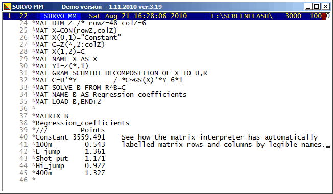
The automatic labelling of matrix rows and columns has been possible already in the matrix interpreter of SURVO 76 (in 1977). It is important to notice the rules for labels in derived matrices. For example, labels are transposed not only when transposing a matrix but also when matrix is inverted, etc. A simple label 'algebra' ensures that in the matrix of regression coefficients the names of regressors appear as row labels and the names of regressands as column labels.
Shakespeare's 154 Sonnets were imported from
http://www.shakespeares-sonnets.com.
The same textual data is studied in demos
Letter frequencies in Shakespeare's Sonnets and
Shakespeare's Sonnets as a Markov chain.
The most important tools were the WORDS, STAT, and SORT commands.
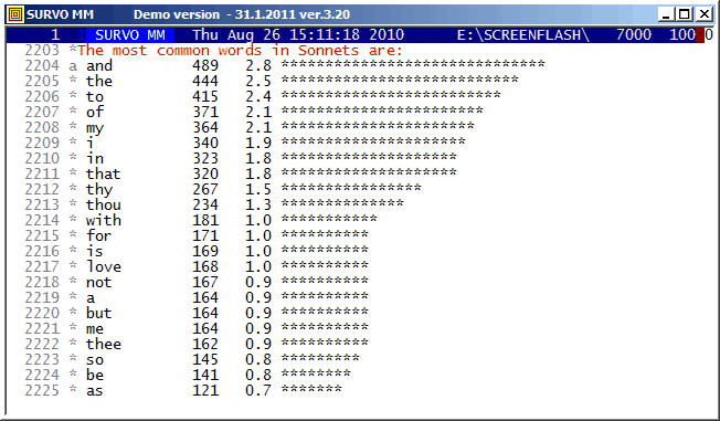
The order of the most common words differs from that of common English for obvious reasons.
One of those commands is
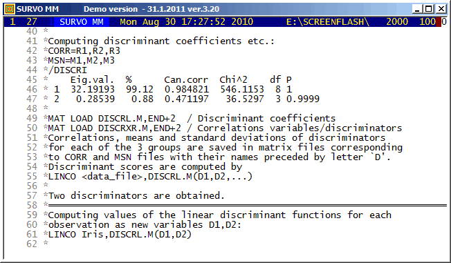
MAT LOAD DISCRXR.M,END+2 / Correlations variables/discriminators
giving in this case
MATRIX DISCRXR.M
Correlations_between_variables_and_discriminators
///        Discr1   Discr2
Sepal_L  -0.79189 -0.21759
Sepal_W   0.53076 -0.75799
Petal_L  -0.98495 -0.04604
Petal_W  -0.97281 -0.22290
and shows that the dominant dicriminator depends essentially on the petal size of the flower.
The discriminant scores were computed by a
LINCO command
LINCO Iris,DISCRL.M(D1,D2)
(as suggested by /DISCRI).
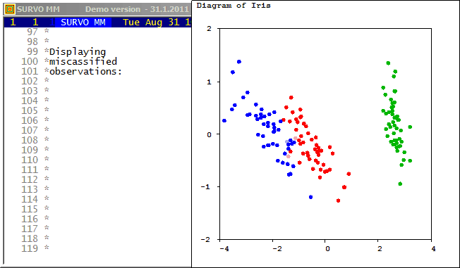
The same data is studied in Cluster analysis of Iris flower data set. by classifying the observations into three groups without any prior information about the species of flowers. It turns out that then clustering according to Wilks' Lambda criterion will be identical to that obtained by reclassification of the original observations according to Mahalanobis distances after discriminant analysis.
Pekka Korhonen has presented an effective stepwise procedure for
computation of lambda values in his doctoral thesis "A stepwise
procedure for multivariate clustering", Computing Centre, University of
Helsinki, Research Reports N:o 7 (1979).
In Korhonen's research a pivot operation plays an essential part
in a form presented earlier by Hannu Väliaho in his doctoral thesis
"A synthetic approach to stepwise regression analysis",
Comm.Phys.Math., vol.34, No.12, 91-132 (1969).
In the CLUSTER program of Survo, the dual procedure of Korhonen's stepwise method is applied. I was Korhonen's opponent in his dissertation and then I took a task to check his algorithms by implementing them to Survo.
This demo in YouTube
This demo in YouTube
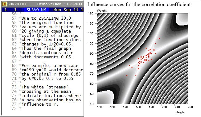
The plotting setup
PLOT z(x,y)=abs(r*(1-w)+u*v)/w
  u=sqrt(n/(n*n-1))*(x-mx)/sx   means mx,my
  v=sqrt(n/(n*n-1))*(y-my)/sy   standard deviations sx,sy
  w=sqrt((1+u*u)*(1+v*v))
TYPE=CONTOUR SCREEN=NEG ZSCALING=20,0
I presented this example among others in my
talk
about Survo in Compstat 1992 (Neuchâtel).
This graph was used by the organizers
of Compstat as a cover page (upside down!!)
in the proceedings of the symposium.

See also
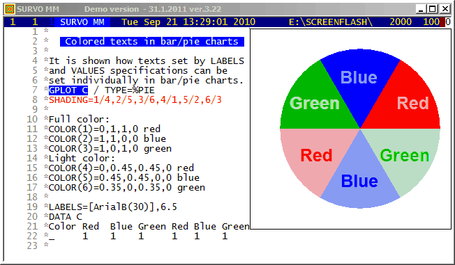
The colors to be used are defined by COLOR(n) specifications telling the color components of each SHADING value n according to the CMYK color model.
The user may edit soft buttons and also create new ones while using Survo.
The default set of soft buttons is defined in the edit field
<Survo>\U\SUR-SOFT.EDT specifying, for example,
the main button line EXIT in the form:
The first Survo Editor (1979) was originally programmed for input
and editing of musical manuscripts and for converting them into
a printable form. The slurs (arched curves connectiong a group of
notes) were then plotted as slightly modified cycloids.
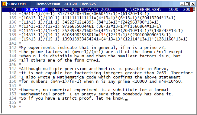
It seems that, in general, numbers of type m^n-1 typically have many (and sometimes all) prime factors of the form c*n+1. By plain numerical calculations I have tried to study their abudance and found some systematic results reported in my paper. These results may have been proved already before. Thus if somebody knows about such proofs, please, let me know.
Editorial computing in Survo makes inventing and testing of this kind of numerical hypotheses easy and comfortable according to the style used in this demo. Making of suitable sucros (Survo macros) is also helpful. The most important sucro /MPN used in this connection has the following listing in a Survo edit field:
*TUTSAVE MPN
/ /MPN m_max,n                              / SM 4.12.2010
/ assuming that n is a prime number
/ computes the prime factors of numbers (m^n-1)/(m-1) for
/ m=2,3,...,m_max
/ and represents them in the form c*n+1.
/ If m-1 divides n, the smallest factor is n.
/
/ See: ../papers/MustonenPrimes.pdf
/
/ def Wmax=W1 Wn=W2 Wm=W3 Wprod=W4 Wc=W5 Wfactor=W6 Wpow=W7
/
*{init}{tempo 0}{disp off}{Wm=2}{R}
*int(exp(log(9000000000000000)/{print Wn}))={act}{l} {save word Wc}
*{line start}{erase}{u}{disp on}{tempo 2}
- if Wmax <= Wc then goto A
*{Wmax=Wc}
+ A: {R}
*({print Wm}^{print Wn}-1)/({print Wm}-1)={act}{l} {line end}
*(10:factors)={act}
/ Remove text "(10:factors)=":
*{l13}{del12}{r}{ref set 1}
/
*{save line Wprod}{erase}{R}{print Wprod}{line start}
/ Replace *'s by spaces:
+ B: {r}{save char Wc}
- if Wc '=' {sp} then goto C
- if Wc '<>' * then goto B
/ Replace * by a space:
* {goto B}
+ C:
/ Each factor to a separate line:
*{home}{u}{ins line}TRIM 1{act}{del line}{home}
*{save char Wc}
- if Wc '<>' {sp} then goto D
*{del line}
/
+ D: {save word Wfactor}{Wpow=1}
- if Wfactor = 0 then goto G
- if Wfactor > Wn then goto D1
/ Wfactor is n
*{form}{goto F}
+ D1:
/ Search for ^
+ D2: {r}{save char Wc}
- if Wc '=' ^ then goto D3
- if Wc '<>' {sp} then goto D2 else goto D4
+ D3:  {save word Wpow}{home}{save word Wfactor}
+ D4: {line start}{erase}({print Wfactor}-1)/{print Wn}={act}
/
*{l} {save word Wc}{line start}{erase}({print Wc}*{print Wn}+1)
/
*{line start}{save word Wfactor}
+ F: {ref jump 1}{write Wfactor}
- if Wpow = 1 then goto F2
*^{print Wpow}
+ F2: *{ref set 1}{R}{del line}{goto D}
+ G: {ref jump 1}{l}{del}
/
- if Wm = Wmax then goto E
*{Wm=Wm+1}{goto A}
+ E: {end}
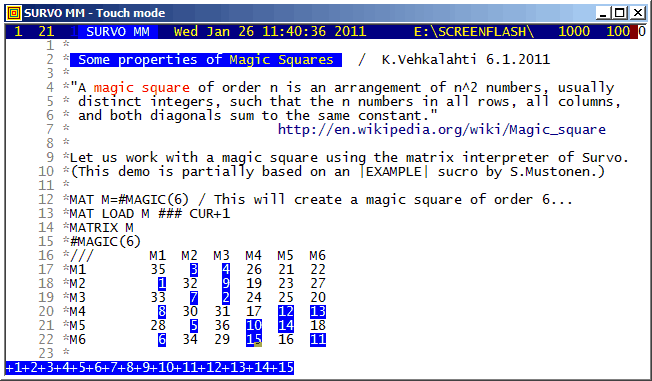
This demo is created by Kimmo Vehkalahti.
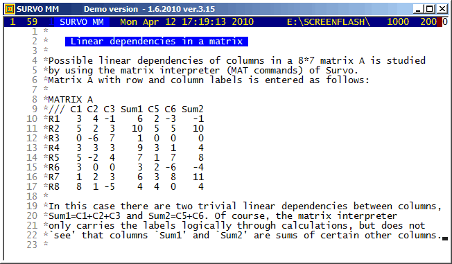
Functions of the Survo matrix interpreter are shown in connection with Magic Squares.
This demo is created by Kimmo Vehkalahti.
Functions of the Survo matrix interpreter are shown in connection with Magic Squares.
A system of linear equations
X1+X2=27
X2+X3=32
X3+X4=32
X1+X3=25
is represented as a matrix equation A*X=B by saving matrices
MATRIX A
///  X1 X2 X3 X4
r12   1  1  0  0
r23   0  1  1  0
r34   0  0  1  1
r13   1  0  1  0

MATRIX B
/// freq
r12   27
r23   32
r34   32
r13   25
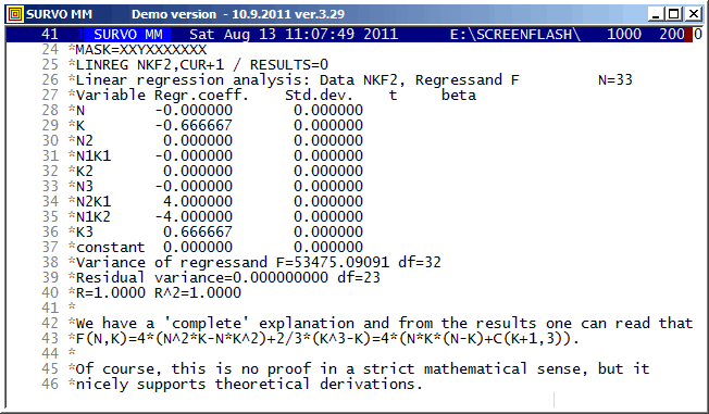
In this example, polynomial regression is applied for determining unknown coefficients of a certain polynomial of two variables from a sample of values.
Originally, this calculation was presented in my
note (in Finnish) (2004)
related to computation of a distribution of
the city block distance
D between two random points in a grid of N x N points.
F(N,K)/N^4 is then the probability P[D=K] for K=1,2,...,N-1.
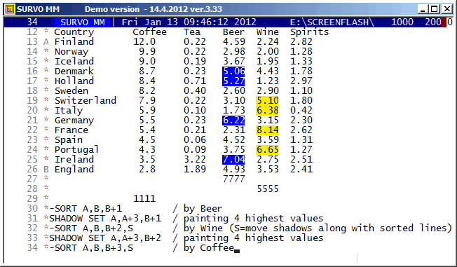
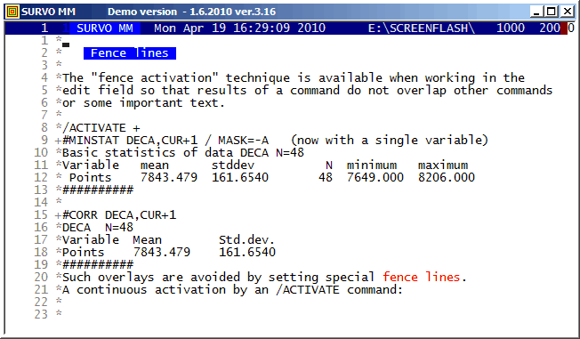
Survo has certain tools for management of shadow lines. The SHADOW SET command is the most recent one (included at the end of year 2011). It enables filling columns of tables with selected shadow characters thus enhancing their appearance.
In fact, this new SHADOW SET does exactly the same job for the shadow lines as the 'classic' SET command for ordinary edit lines.
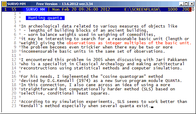
Our task is to estimate the values of quanta q_1, q_2,..., q_k on the condition that each of them exceeds a certain minimum value q_min.
D.G.Kendall has in his paper Hunting Quanta (Royal Society of London. Mathematical and Physical Sciences A 276, 231-266) proposed using a "cosine quantogram" of the form
                         n
    phi(q) = sqrt(2/n)* SUM cos(2*pi*eps(i)/q)                (Kendall 1974)
                        i=1
My idea is that the quanta are estimated by a selective, conditional least squares method where the sum
                      n
   ss(q_1,...,q_k) = SUM min[g(x_i,q_1)^2,...,g(x_i,q_k)^2]       (SLS 2005)
                     i=1
A more detailed description is found in my paper Hunting multiple quanta by selective least squares.
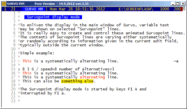
All Survopoint lines are indicated by the '~' (tilde) character in the control column. At the end of such a line a marking of type ~x must exist. x is any of the lowercase characters a,b,...,z. For any x, a line having x in its control column must exist in the same edit field (typically outside the Survo window) and this line tells how the corresponding Survopoint line is displayed.
For example, in this demo the display mode of English proverbs (appearing in the latter part of the demo) is defined as follows:
e 30 159 S
*    The road to hell is paved with good intentions.
*    He laughs best who laughs last.
*    A smooth sea never made a skilled mariner.
*    Truth is stranger than fiction.
*    A friend to all is a friend to none.
*    Be swift to hear, slow to speak.
*    Knowledge in youth is wisdom in age.
 ...
On the 'e' line, 30 indicates the rate of change (this Survopoint line is altered only once in 30 sequent refreshments of the display). 159 is the number of proverbs in the list and 'S' indicates a systematic change.
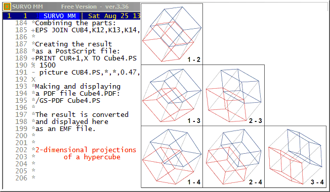
One of the illustrations is a graph of a 4-dimensional cube represented as 2-dimensional projections. This graph resembles a draftsman's plot (scatterplot matrix) of multivariate statistical data.
Here this graph is generated by a series of Survo operations triggered by an /ACTIVATE sucro command. Below is a complete description (an extract from a Survo edit field) about how the graph has been created:
 65 *
 66 *The following sucro command activates all commands having a '+' in the
 67 *control column and thus the final graph will be automatically created:
 68 *
 69 */ACTIVATE +  (Activated commands are displayed here in red.)
 70 *It is possible to draw each 2-dimensional projection of a 4-dimensional
 71 *cube as a single line graph of edges since the degree of each vertex
 72 *is 4. Then there exists an Eulerian circuit where each edge is
 73 *traversed just once.
 74 *Consider the cube in a 4-dimensional space so that vertices have
 75 *coordinates (x_1,x_2,x_3,x_4) where each x_i is either 0 or 1.
 76 *Then the following matrix gives an Eulerian circuit in this
 77 *4-dimensional cube:
 78 *
 79 *MATRIX C4 ///
 80 *0 0 0 0
 81 *0 0 0 1
 82 *0 0 1 1
 83 *0 0 1 0
 84 *0 0 0 0
 85 *0 1 0 0
 86 *0 1 0 1
 87 *0 1 1 1
 88 *0 1 1 0
 89 *0 1 0 0
 90 *1 1 0 0
 91 *1 1 0 1
 92 *0 1 0 1
 93 *0 0 0 1
 94 *1 0 0 1
 95 *1 1 0 1
 96 *1 1 1 1
 97 *0 1 1 1
 98 *0 0 1 1
 99 *1 0 1 1
100 *1 0 0 1
101 *1 0 0 0
102 *1 1 0 0
103 *1 1 1 0
104 *0 1 1 0
105 *0 0 1 0
106 *1 0 1 0
107 *1 0 1 1
108 *1 1 1 1
109 *1 1 1 0
110 *1 0 1 0
111 *1 0 0 0
112 *0 0 0 0
113 *
114 +MAT SAVE C4
115 +MAT TRANSFORM C4 BY X#-0.5   / Centering (0,1) -> (-0.5,0.5)
116 +MAT CLABELS "X" TO C4        / Column labels X1,X2,X3,X4
117 *
118 *The regular 2-dimensional projections of this hypercube are plain
119 *squares and thus not very interesting.
120 *
121 *A better view is obtained by making an "arbitrary" 4-dimensional
122 *rotation:
123 *
124 +MAT T=ZER(4,4)
125 +MAT TRANSFORM T BY sin(31*I#*J#)  / "arbitrary" T
126 *
127 +MAT GRAM-SCHMIDT DECOMPOSITION OF T TO Q,R  / Orthogonalization of T
128 +MAT K=C4*Q                  / Rotation of the hypercube by orthogonal Q
129 +MAT CLABELS "dim" TO K      / Column labels dim1,dim2,dim3,dim4
130 *
131 *Combining the rotated and original cube into one matrix KB:
132 *
133 +MAT KB=ZER(33,8)
134 +MAT KB(1,1)=K
135 +MAT KB(1,5)=C4
136 *
137 *.......................................................................
138 *Plotting all six 2-dimensional projections separately:
139 *
140 *SIZE=1000,1000 SCALE=-1,1 HEADER= XDIV=0,1,0 YDIV=0,1,0 FRAME=3
141 *FRAMES=F F=0,0,1000,1000 PEN=[SwissB(30)]
142 *XLABEL= YLABEL= LINE=[line_type(2)][line_width(0.2)],1 TEXTS=T
143 *
144 +PLOT KB.MAT,dim1,dim2 / DEVICE=PS,A12.PS T=1_-_2,750,50
145 +PLOT KB.MAT,dim1,dim3 / DEVICE=PS,A13.PS T=1_-_3,750,50
146 +PLOT KB.MAT,dim1,dim4 / DEVICE=PS,A14.PS T=1_-_4,750,50
147 +PLOT KB.MAT,dim2,dim3 / DEVICE=PS,A23.PS T=2_-_3,750,50
148 +PLOT KB.MAT,dim2,dim4 / DEVICE=PS,A24.PS T=2_-_4,750,50
149 +PLOT KB.MAT,dim3,dim4 / DEVICE=PS,A34.PS T=3_-_4,750,50
150 *
151 *.......................................................................
152 *Plotting two opposite 3-dimensional cubes in different colors (blue and
153 *red):
154 *
155 *SIZE=1000,1000 SCALE=-1,1 HEADER= XDIV=0,1,0 YDIV=0,1,0 FRAME=0
156 *XLABEL= YLABEL=
157 *               *blue=[color(1,1,0,0)],1 *red=[color(0,1,1,0)],1
158 +PLOT KB.MAT,dim1,dim2 / DEVICE=PS,B12.PS IND=X1,-0.5 LINE=*blue
159 +PLOT KB.MAT,dim1,dim2 / DEVICE=PS,C12.PS IND=X1,0.5  LINE=*red
160 +PLOT KB.MAT,dim1,dim3 / DEVICE=PS,B13.PS IND=X1,-0.5 LINE=*blue
161 +PLOT KB.MAT,dim1,dim3 / DEVICE=PS,C13.PS IND=X1,0.5  LINE=*red
162 +PLOT KB.MAT,dim1,dim4 / DEVICE=PS,B14.PS IND=X1,-0.5 LINE=*blue
163 +PLOT KB.MAT,dim1,dim4 / DEVICE=PS,C14.PS IND=X1,0.5  LINE=*red
164 +PLOT KB.MAT,dim2,dim3 / DEVICE=PS,B23.PS IND=X1,-0.5 LINE=*blue
165 +PLOT KB.MAT,dim2,dim3 / DEVICE=PS,C23.PS IND=X1,0.5  LINE=*red
166 +PLOT KB.MAT,dim2,dim4 / DEVICE=PS,B24.PS IND=X1,-0.5 LINE=*blue
167 +PLOT KB.MAT,dim2,dim4 / DEVICE=PS,C24.PS IND=X1,0.5  LINE=*red
168 +PLOT KB.MAT,dim3,dim4 / DEVICE=PS,B34.PS IND=X1,-0.5 LINE=*blue
169 +PLOT KB.MAT,dim3,dim4 / DEVICE=PS,C34.PS IND=X1,0.5  LINE=*red
170 *
171 *Coloring the projections:
172 +EPS JOIN K12,A12,B12,C12
173 +EPS JOIN K13,A13,B13,C13
174 +EPS JOIN K14,A14,B14,C14
175 +EPS JOIN K23,A23,B23,C23
176 +EPS JOIN K24,A24,B24,C24
177 +EPS JOIN K34,A34,B34,C34
178 *
179 *Entering coordinates for projections in the final setup:
180 *K12=K12,0,2000
181 *K13=K13,0,1000   K23=K23,1000,1000
182 *K14=K14          K24=K24,1000,0      K34=K34,2000,0
183 *
184 *Combining the parts:
185 +EPS JOIN CUB4,K12,K13,K14,K23,K24,K34
186 *
187 *Creating the result
188 *as a PostScript file:
189 +PRINT CUR+1,X TO Cube4.PS
190 % 1500
191 - picture CUB4.PS,*,*,0.47,0.47
192 X
193 *Making and displaying
194 *a PDF file Cube4.PDF:
195 +/GS-PDF Cube4.PS
196 *
197 *The result is converted
198 *and displayed here
199 *as an EMF file.
200 *
In the
appendix (pp. 181-)
it is also shown e.g. that the number of m-cubes in an n-cube
is K(n,m)=C(n,m)2^(n-m), m=0,1,2,...,n. Thus, for example, the number of
edges in a cube is C(3,1)*2^(3-1)=12 and the number of cubes in a
4-dimensional cube is C(4,3)*2^(4-3)=8. These 8 cubes are shown below
as 2-dimensional projections to first two coordinate axes.
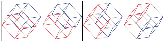
The first pair is the same as in the 1-2 plot defined on lines 157-159 in the template above and the remaining three pairs are obtained by changing X1 on lines 158 and 159 to X2,X3,X4, respectively.
The generating function of K(n,n-m) numbers is f(s)=(s+2)^n in the same way as (s+1)^n is the generating function of the binomial coefficients C(n,m). The total number of "parts": vertices (m=0), edges (m=1), faces (m=2), cubes (m=3), etc. in an n-dimensional cube is then f(1)=(2+1)^n=3^n.

Copies of various items in the edit field can be made in various ways.
For 'words' (contiguous strings separated by blanks) the best method
from version 3.37 onwards is based on two mouse-clicks:
- - - - - - - - - -

See also
http://www.survo.fi/papers/Polygons2013.pdf
http://www.survo.fi/papers/Roots2013.pdf.
and
Mustonen, S., Haukkanen, P., Merikoski, J. (2014).
Some polynomials associated with regular polygons.
Acta Univ. Sapientiae, Mathematica, 6, 2, 178-193.
More extensive demos about the same subject:
Equation for the sum of chord lengths in a regular polygon
Regular polygons: Solving riddle of q coefficients
Regular polygons: Testing roots
This demo in YouTube
This is partial reproduction of my talk
"Editorial approach in statistical computing"
in
the Second International Tampere Conference in Statistics (1987).
This demo gives two examples about usage of Survo.
In the original
video

many details related to these examples are difficult to see.
The last example 'Estimation of a circle' of my talk is also available in YouTube.
The final paper in conference proceedings does not include these examples.
This demo in YouTube
Thurstone's problem is presented in a more general form. Values of the derived variables have substantial 'measurement' errors.
The Thurstone's original experiment is described, for example, in Richard L. Gorsuch: Factor Analysis pp. 10-11.
This demo in YouTube and also as a flash demo.
Although these recursive formulas are more complicated than the direct double sum formula (presented in the beginning) they give results much faster. For example, already when n=10^4 recursive formulas are over 1000 times faster than the double sum formula. Furthermore, the recursive formulas are applied iteratively so that results are obtained at the same time also for all integers less than n and it is efficient to continue iteration for greater n values step by step on the basis of values L(n,n), L(n-1,n), and R1(n).
By these means I have computed L(n,n) values for all n <= 10^8 in 100 sequences of a million n values and it would take less than 3 hours on my current PC. The same task by using the double sum formula would last over 100'000 years!
In 2015 I extended this calculation for all n <= 10^11.
More information about this topic is given in Grid lines where the asymptotic behaviour of L(n,n) numbers is reported.
See also
This demo in YouTube
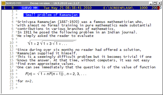
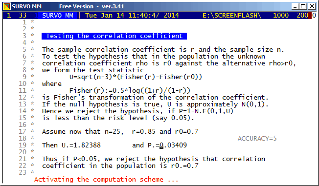
This is one of the oldest examples (in 1981)(see page 59) used for demonstrating 'self-documenting' and 'literate programming' in the Survo Editor. These terms were unknown to me since apparently they were introduced later e.g. by Donald Knuth.
It should be noted that all information (formulas and data) needed for computation of test statistics is given within the text typed in the edit field.
This demo in YouTube
This demo was a part of my talk
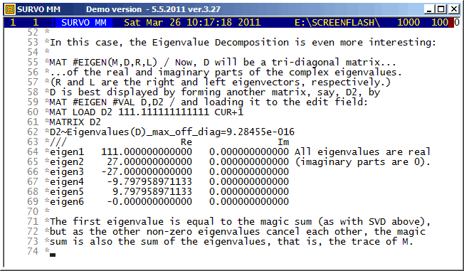
Matrix computations in Survo
in The Eighth International Workshop on Matrices and Statistics (1999)
at the University of Tampere, Finland.
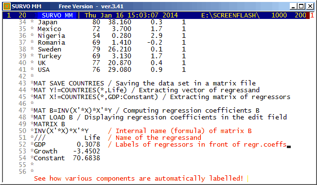
It is easy to convert a matrix file to a Survo data file by
FILE SAVE MAT <matrix_file> TO <Survo_data_file>and conversely any Survo data (table or file) to a matrix file by
MAT SAVE DATA <Survo_data> TO <matrix_file>but Survo matrix files (like COUNTRIES.MAT in this demo) can be used also as data in statistical operations.
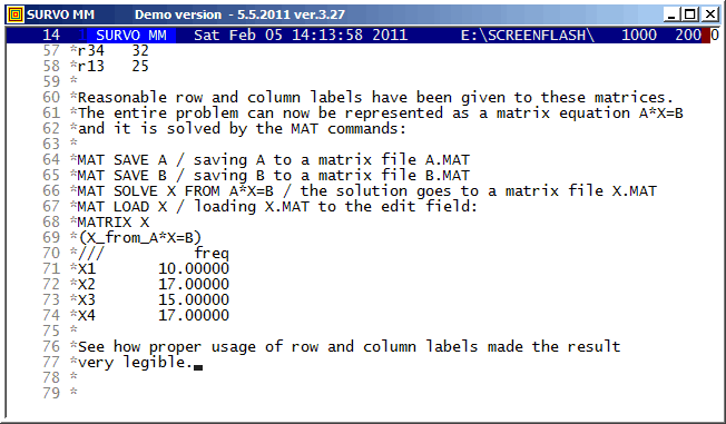
The matrix interpreter is also useful for teaching methods related to linear models, for example.
The automatic labelling of matrix rows and columns has been possible already in the matrix interpreter of SURVO 76 (in 1977). It is important to notice the rules for labels in derived matrices. For example, labels are transposed not only when transposing a matrix but also when matrix is inverted, etc. A simple label 'algebra' ensures that in the matrix of regression coefficients the names of regressors appear as row labels and the names of regressands as column labels.
This demo in YouTube
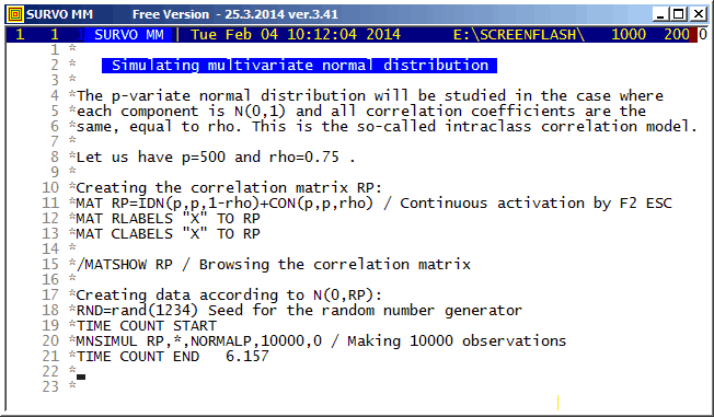
GPLOT x(t)=X0+R*(sin(t)+r*sin(A*t)+r^2*sin(B*t)),
      y(t)=Y0+R*(cos(t)+r*cos(A*t)+r^2*cos(B*t))

r=(sqrt(5)-1)/2 s=1/(1+r+r^2) R=3*r/2
t=0,2*pi,pi/1000 pi=3.141592653589793
SCALE=-4,4 OUTFILE=A
XDIV=0,1,0 YDIV=0,1,0 SIZE=381,381 HEADER= FRAME=3 MODE=381,381
i=0(1)3
a=5
b=15 T1=5;15,170,170 TEXTS=T1
PEN=[color(0.2,0.4,1,0)][SwissB(20)]
FILL(-2)=0.9,0.6,0.3,0
LINETYPE=[line_width(2)],1 SLOW=300
A=x0*a+1  X0=2*x0  x0=int(sqrt(2)*(sin(pi/2*(i+0.5)))+0.5)
B=y0*b+1  Y0=2*y0  y0=int(sqrt(2)*(cos(pi/2*(i+0.5)))+0.5)
WSIZE=381,381 WHOME=800,0 WSTYLE=0 FRAMES=F F=0,0,381,381,-2

The setup of graphs corresponds to values (here A=5, B=15) in this way:
      -A,B    A,B

      -A,-B   A,-B
MATRIX AB
///  a  b C     M     Y     c     m     y     L  W   S
  1  5 15 0.200 0.400 1.000 0.900 0.600 0.300 1 40 300
  2  0  0 1.000 1.000 1.000 0.000 0.000 0.000 1  7  50
  3  1  1 1.000 1.000 1.000 0.000 0.000 0.000 1  4  20
  4  2  2 1.000 1.000 1.000 0.000 0.000 0.000 1  3  10
  5  3  3 1.000 1.000 1.000 0.000 0.000 0.000 1  2   5
... .. .. ..... ..... ..... ..... ..... ..... . .. ...
 95  9  7 0.298 0.498 1.000 0.872 0.605 0.204 1  1   0
 96  9 15 0.260 0.397 1.000 0.858 0.655 0.175 1  1   0
 97 11 32 0.323 0.374 1.000 0.917 0.711 0.211 1  1   0
 98 16 96 0.313 0.427 1.000 0.838 0.537 0.237 1  1   0
 99 45 50 0.170 0.401 1.000 0.918 0.640 0.245 1  8 100
100 10 60 1.000 1.000 1.000 0.000 0.000 0.000 1 25 300
This demo in YouTube
This is a replicate of a my flash demo created in 2006. The most significant distinction is that the computation times (including loading and saving) measured in Survo by TIME COUNT START - TIME COUNT END commands were now only about a third of those obtained eight years earlier. There are no changes in the program code but PC's have become somewhat faster.
This demo in YouTube
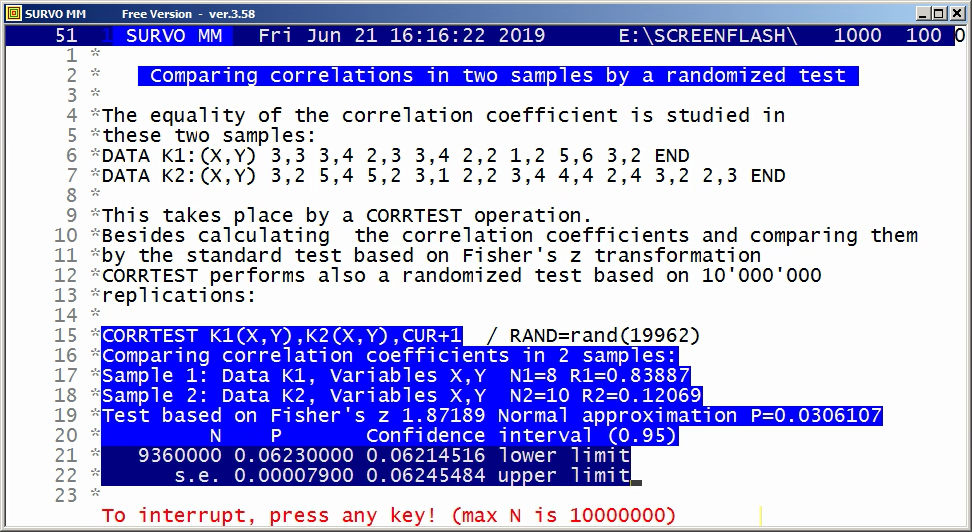
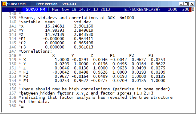
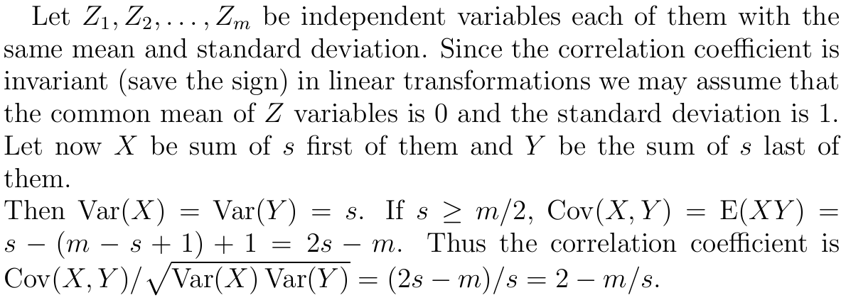
Throughout the calculations the matrix interpreter of Survo is used.
The simple formula for the correlation coefficient in the current case is derived as follows:
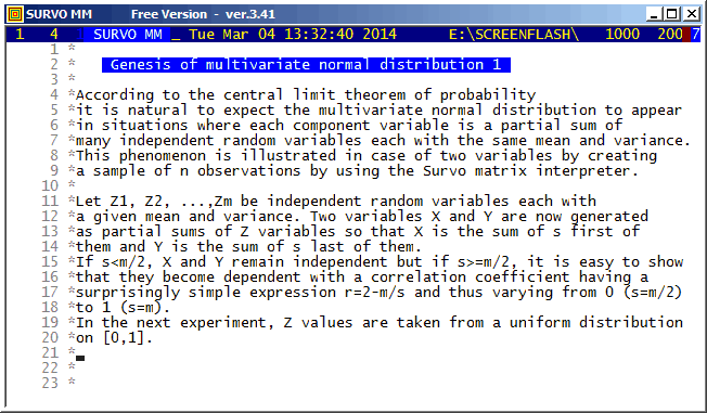
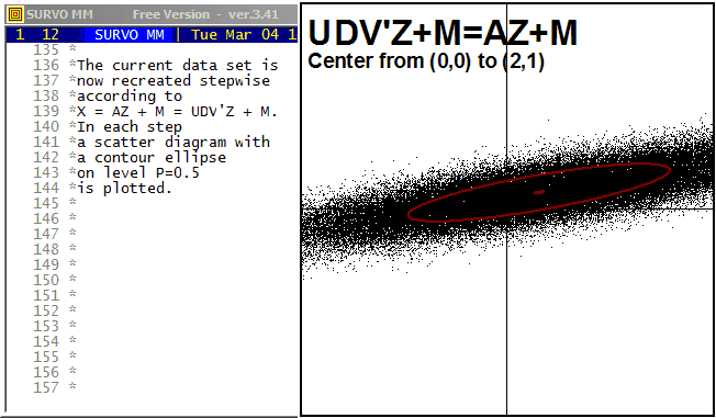
According to my experience, in general, the most clear-cut way to define multivariate normal distribution is by a linear transformation of independent N(0,1) variables.
This demo in YouTube
For example, from this standpoint one can readily understand that there can be only linear dependencies between component variables, or see that its marginal and conditional distributions are (multi)normal.
In my lecture notes (1995) on multivariate statistical methods (in Finnish) almost everything is derived on this basis without a need for working with integrals, etc. The creation of two-dimensional normal normal distribution is characterized there (p.16) in this way
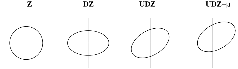
The main tool in calculations is here the matrix interpreter of Survo.
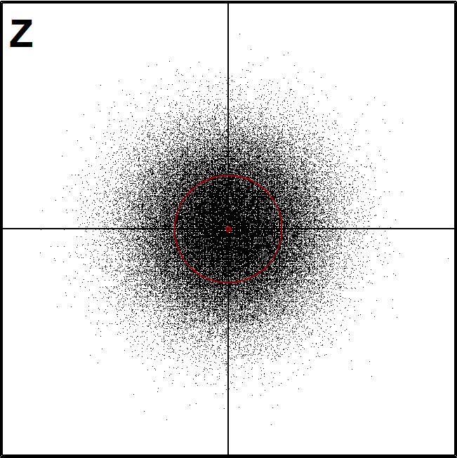
Graphics were generated by Survo plotting schemes in the following way:
(here the first figure Z of a sample of N2(0,I) distribution)
*
*Matrix Z of independent N(0,1) variables:
*MAT Z=ZER(100000,2)              / Z is a data frame.
*MAT #TRANSFORM Z BY #RAND(20140) / Fill with uniform[0,1] values,
*MAT #TRANSFORM Z BY probit(X#)   / convert to independent N(0,1) values
*
A Common specifications:
*WHOME=271,0 WSIZE=381,381 HEADER= XDIV=0,1,0 YDIV=0,1,0 XLABEL= YLABEL=
*WSTYLE=0 FRAME=3 LINETYPE=[line_width(3)],1 POINT=11 MODE=1024,1024
*SCALE=-5,5
B
*..................................
*Coordinate axes: (common backgroud for each graph)
*GPLOT X(t)=c*t,Y(t)=(1-c)*t / SPECS=A,B
*c=0,1,1 t=-9,9,9
*OUTFILE=Z0
*..................................
*Scatter diagram of two independent N(0,1) variables, 100'000 cases
*GPLOT Z.MAT,1,2 / SPECS=A,B CONTOUR=[RED],0.001,0.5
*PEN=[BLACK][SwissB(100)] TEXTS=T T=Z,20,900
*INFILE=Z0 OUTFILE=Z1
*
A related demo: Genesis of multivariate normal distribution 1
This demo in YouTube
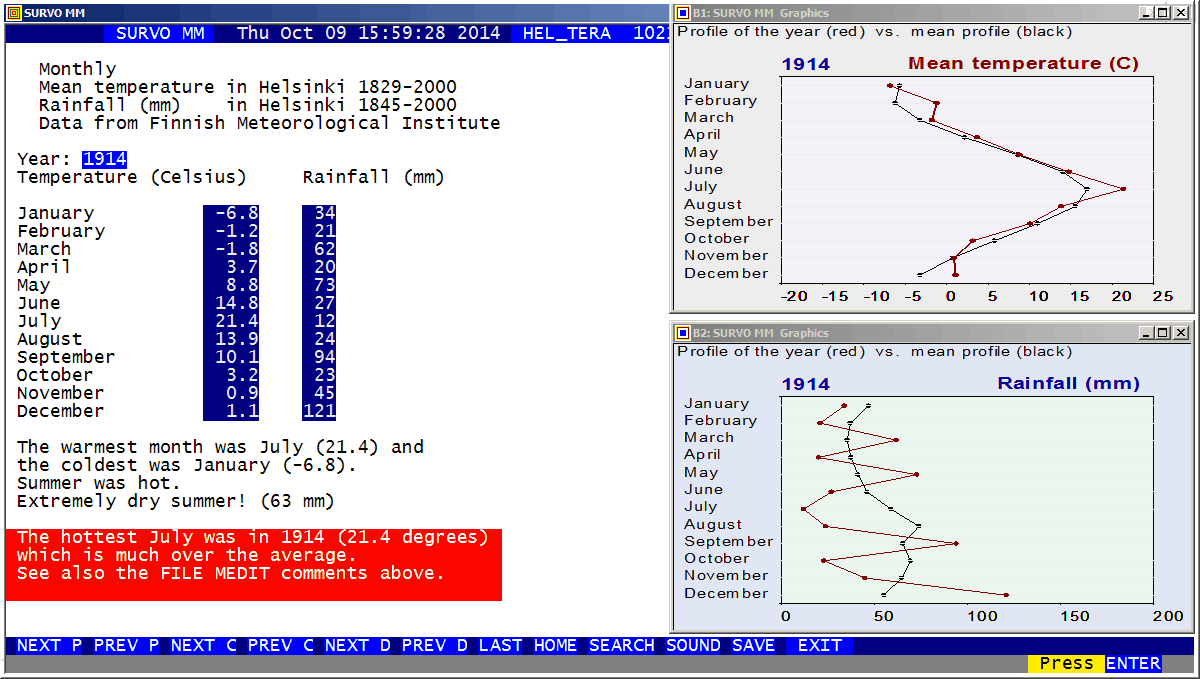
In the second half of this demo (displaying graphs), another Survo session is called to create graphics by PLOT commands. The instructions for the entire application are given in an edit field HELTERA3.EDT
This demo in YouTube
This was a useful feature because at that time a typical statistical analysis would take a long time, often more than ten minutes, and one learned to recognize the various stages of standard programs just by listening the sound.
During my summer holiday in 1962 I decided to create a program just for producing sound sequences created more or less randomly. The program included subroutines for random 'trills' and 'glissandos', for example. It was also able to make random 'variations' on a 'theme' given by the operator from the keyboard or by the program itself.
It may have been the first program for both generating 'music' and playing it in real time. I had a rough estimate that it would take about 10^50 years before the program starts to repeat itself ☺.
The most serious drawback was that the highest tone
was only about H=1135 Hz (caused by the shortest possible loop) and all
other tones were H/2, H/3, H/4, ... Hz so that the scale of tones
was primitive indeed.
This example contains small captions of the sound output generated
by this program. The samples were taken by Erkki Kurenniemi on a recorder
of the Department of Music in the University of Helsinki in 1962.
They are now available on a CD "On-Off" produced by Petri Kuljuntausta.
See also
Peter Onion's video
about my program in YouTube. In this video the program code punched
on a paper tape is fed into the ferrite core memory of Elliott 803
and the program starts
immediately thereafter according to default settings.
This demo in YouTube
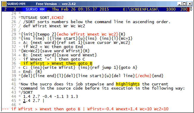
*TUTSAVE SORT
/ /SORT sorts numbers below the command line in ascending order.
/ Defining variables:
/ def Wfirst Wnext Wr Wc Wc2
/
/ Initialization and setting maximum speed:
*{init}{tempo 0}
*
/ Making room for the sorted list:
*{R}{ins line}
/
/ Setting a 'wall' |:
* |
/
/ Setting a space in front of the original list:
*{line start}{u}{ins} {ins}{l}{Wc=1}
/
/ Finding next number and recording its location:
+ A: {next word}{ref set 1}{save cursor Wr,Wc2}
/
/ If no next number found, going to End:
- if  Wc2 = Wc then goto End
/
/ Saving new number:
*{Wc=Wc2}{save word Wfirst}{R}
/
/ Finding next word on result line:
+ B: {next word}{save word Wnext}
/
/ If it is the wall, inserting value of Wnext to the end:
- if Wnext '=' | then goto C
/
/ Repeating from B if proper location for Wfirst not yet found:
- if Wfirst > Wnext then goto B
/
/ Writing newest number to its place in the sorted list:
+ C: {ins}{write Wfirst} {ins}{ref jump 1}{goto A}
/
/ Finishing by removing the wall and the original list:
+ End: {R}{del}{line end}{l}{del}{line start}{u}{del line}
*{end}
This demo in YouTube
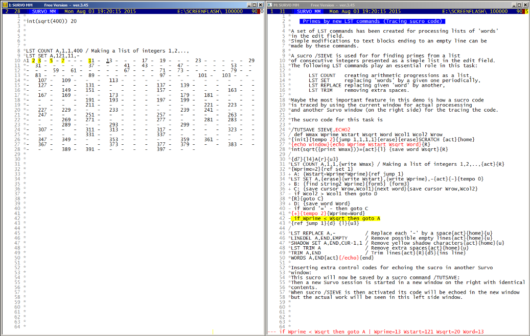
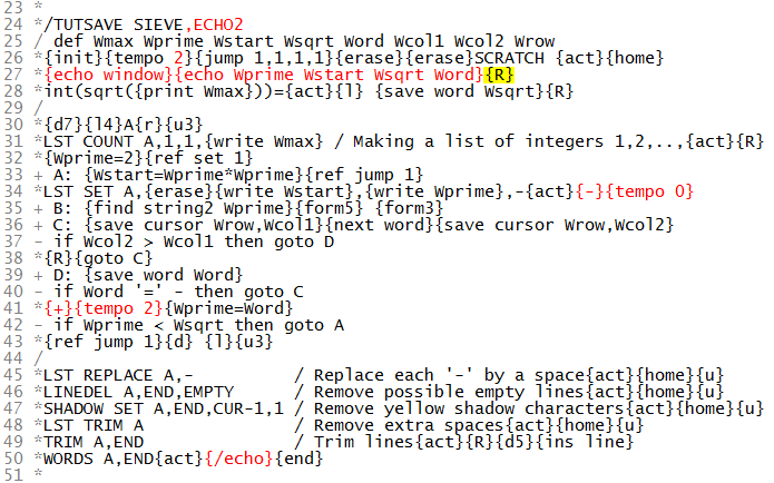
That command appears on the line 33 above in the form
SET A+{write Wstart},A+{write Wmax},A,{write Wprime}
and it takes actual forms
SET A+4,A+1000000,A-1,2
SET A+9,A+1000000,A-1,3
SET A+25,A+1000000,A-1,5
SET A+49,A+1000000,A-1,7
in the four first rounds.
The speed of this process is much higher than in the older example, but even here the fact that integers are represented as character strings and converted to double precison floating point numbers slows down the computation dramatically.
Thus in pure numerical computations the sucro technique is inefficient. Sucros are at their best when makining tutorials like these demos or when the task at hand is a sequence of standard Survo operations and the same job has to be repeated many times from various initial conditions. See, for example Combining Survo operations by sucros
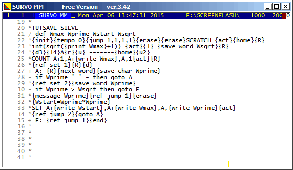
This approach is very slow when compared to a corresponding task
carried out by a pure C program presented as a Survo command SIEVE
below. Finding of all primes below a million and loading them to the
edit field (see lines 80- in the C code below) takes only 0.245 seconds
and is thus about 100 times faster.
More about programming Survo in C

    1 *SAVE SIEVE
    2 *
    3 a/* _sieve.c 8.4.2015/SM (8.4.2015) */
    4 *
    5 *#include <stdio.h>
    6 *#include <stdlib.h>
    7 *#include <malloc.h>
    8 *#include <math.h>
    9 *#include <survo.h>
   10 *#include <survoext.h>
   11 *
   12 *unsigned int n;
   13 *char *prime;
   14 *int j,h;
   15 *
   16 *void main(argc,argv)
   17 *int argc; char *argv[];
   18 *    {
   19 *    unsigned int i,n,max,p,count,output;
   20 *    if (argc==1) return;
   21 *    s_init(argv[1]); // initializing Survo environment for this program
   22 *    if (g<2)
   23 *        {
   24 *        sur_print("\nUsage: SIEVE N [output=0,1,2]");
   25 *        WAIT; return;
   26 *        }
   27 *    n=atoi(word[1]);
   28 *    prime=(char *)malloc(n+1); // reserving space for prime indicators
   29 *    for (i=0; i<n+1; ++i) prime[i]='1'; // at the start all are primes
   30 *    max=(int)sqrt((double)n);  // max number to be tested is sqrt(n)
   31 *    p=1; output=2;
   32 *    if (g>2) output=atoi(word[2]); // selecting scope of output
   33 *    while (p<max)
   34 *       {
   35 *       ++p;
   36 *       while (prime[p]=='0') ++p; // finding next prime p
   37 *       for (i=p*p; i<=n; i+=p) prime[i]='0'; // multiples of p composite
   38 *       } // all primes found
   39 *    count=0;
   40 *    j=r1+r; new_line();
   41 *    for (i=2; i<n+1; ++i)
   42 *       if (prime[i]=='1')
   43 *          {
   44 *          ++count; // counting number of primes
   45 *          if (output==2)
   46 *              {
   47 *              h+=sprintf(sbuf+h,"%u ",i); // collecting primes on a line
   48 *              if (h>c-7) // visible line length - 7
   49 *                  {
   50 *                  out();
   51 *                  new_line();
   52 *                  }
   53 *              }
   54 *          }
   55 *    if (output>0)
   56 *          {
   57 *          if (output==2) out();
   58 *          new_line();
   59 *          sprintf(sbuf,"Number of primes < %u is %u.",n,count);
   60 *          out();
   61 *          s_end(argv[1]); // output to be catched by the editor
   62 *          }
   63 *    return;
   64 *    }
   65 *
   66 *new_line()
   67 *    {
   68 *    ++j; h=0; *sbuf=EOS; // output=2
   69 *    return(1);
   70 *    }
   71 *
   72 *out()
   73 *    {
   74 *    edwrite(space,j,1);
   75 *    edwrite(sbuf,j,1);
   76 *    return(1);
   77 *    }
   78 A
   79 *
   80 *TIME COUNT START / Continuous activation by F2 ESC
   81 *SIEVE 1000000
   82 *TIME COUNT END   0.245
   83 *2 3 5 7 11 13 17 19 23 29 31 37 41 43 47 53 59 61 67 71 73 79 83 89
   84 *97 101 103 107 109 113 127 131 137 139 149 151 157 163 167 173 179
   85 *181 191 193 197 199 211 223 227 229 233 239 241 251 257 263 269 271
   86 *277 281 283 293 307 311 313 317 331 337 347 349 353 359 367 373 379
   87 *383 389 397 401 409 419 421 431 433 439 443 449 457 461 463 467 479
   88 *487 491 499 503 509 521 523 541 547 557 563 569 571 577 587 593 599
   89 *601 607 613 617 619 631 641 643 647 653 659 661 673 677 683 691 701
   90 *709 719 727 733 739 743 751 757 761 769 773 787 797 809 811 821 823
   91 *827 829 839 853 857 859 863 877 881 883 887 907 911 919 929 937 941
   92 *947 953 967 971 977 983 991 997 1009 1013 1019 1021 1031 1033 1039
   - - - - - - - - - - -
 7817 *999529 999541 999553 999563 999599 999611 999613 999623 999631 999653
 7818 *999667 999671 999683 999721 999727 999749 999763 999769 999773 999809
 7819 *999853 999863 999883 999907 999917 999931 999953 999959 999961 999979
 7820 *999983
 7821 *Number of primes < 1000000 is 78498.
 7822 *
This demo in YouTube
This as flash demo
For example, the entire sucro code of this demo is:
11 *
12 */M
13 *TUTSAVE M
14 *{tempo -1}{init}{jump 1,1,1,1}SCRATCH {act}{line start}
15 /
16 *COLX W20{act}{line start}{erase}{tempo 2}{wait 100}{tempo -1}
17 *{R}
18 * {form7} Combining Survo operations by sucros {R}
19 *{R}
20 *Sucros are at their best when the task at hand is a sequence of{R}
21 *standard Survo operations and the same job has to be repeated{R}
22 *many times from various initial conditions.{R}
23 *For example, sucros have been created for performing some multistage{R}
24 *forms of statistical analysis.{R}
25 *Here a sucro /FACTOR is presented. It carries out the standard steps{R}
26 *of factor analysis:{R}
27 *{R}
28 *1. Computing correlations CORR.M{R}
29 *2. Computing eigenvalues by spectral decomposition of CORR.M{R}
30 *3. The number of factors f is determined as follows:{R}
31 * Eigenvalues e(1)>=e(2)>=e(3)>=...{R}
32 * Ratios s(i)=e(i+1)/e(i), if e(i)>=0.9, s(i)=1 else{R}
33 * Let e(j)>=1 and e(j+1)=<1 and s(k)=min(s(j),s(j+1),s(j+2)){R}
34 * Then f=k.{R}
35 *4. Computing the maximum likelihood solution FACT.M by FACTA{R}
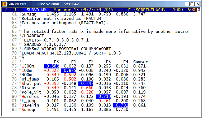
36 *5. Computing the rotated factor matrix AFACT.M by ROTATE{R}
37 *{R}
38 */FACTOR is now applied to the dataset DECA on the 48 best athletes{R}
39 *of the world in 1973.
40 /
41 *{tempo 2}{90}{R}
42 *{d5}{tempo 0}{d14}{u19}{tempo 2}{10}
43 *
44 *The 10 event{tempo 0} variables will be considered
45 * and thus set active in DECA:{tempo 2}{20}{R}
46 *FILE ACTIVATE DECA{keys 2}{act}
47 /
48 *--AAAAAAAAAA--{exit}
49 /
50 *{keys 0}{10}{R}
51 *Sucro /FACTOR{tempo 0} is activated with dataset DECA:
52 *{tempo 2}{10}{R}
53 */FACTOR DECA{keys 2}{act}{keys 0}{30}
54 *
55 *{d14}{20}{d14}{20}{del line}{d21}{u18}{10}
56 /
57 *The rotated{tempo 0} factor matrix is made
58 * more informative by another sucro:{tempo 2}{20}
59 *{R}
60 */LOADFACT{keys 2}{act}{keys 0}{30}
61 /
62 *{d17}{u2}
63 *Typically{tempo 0} for Survo, the work has documented itself and it may be {R}
64 *repeated.{tempo 2}{20}
65 * Now e.g. {tempo 0}a four-factor solution can be obtained 'manually'
66 *{R}
67 *and another rotation technique can be adopted:
68 *{tempo 2}{30}{home}{5}{u55}{5}{r13}{10}4{r}35 {keys 2}{act}{keys 0}
69 /
70 *{10}{d}{l6}4{r}49{erase}{5} / ROTATION=ORTHO_CLF (by Jennrich)
71 *{keys 2}{act}{keys 0}{10}{R}
72 *{d28}{20}{d22}{u13}{10}SCRATCH{10}{act}{10}{R}
73 *{u2}{keys 2}{act}{keys 0}{end}
74 *
In sucros intended for teaching or demonstrating it is important to regulate timing of the process. This takes place by wait codes ( {wait 20} or simply {20} means a wait for two seconds ) and tempo codes ( {tempo 0} sets the fastest speed for 'writing' and {tempo 2} a normal speed ).
An essential part of sucro programming is the 'cursor choreography' i.e. how the cursor is moved in the edit field. Also this sucro contains plenty of codes like {d14} (14 steps downwards) or {r6} (6 steps to the right).
The keys codes control echoing of key strokes in the lower right corner of the Survo window. {keys 2} starts echoing and {keys 0} cancels it. This property is used on lines 46-50 when selecting active variables from DECA and in most activations of Survo commands.
Sucro /FACTOR used here as a 'subroutine' has a different nature as
a tool for a rapid automatic execution of the typical stages of factor
analysis. There are also conditional statements for determination
of the number of factors, for example.
 11 *
 12 *TUTLOAD <Survo>\S\FACTOR
 13 /    /FACTOR <data>                         / 10.6.1991/SM (13.5.1994)
 14 / or /FACTOR <data>,<number_of_factors>
 15 *{tempo -1}{init}{R}
 16 *SCRATCH {act}{home}
 17 - if W1 '=' ? then goto A
 18 - if W1 '<>' (empty) then goto S
 19 + A: /FACTOR <data>{R}
 20 *makes a factor analysis from active variables and observations of{R}
 21 *a Survo data <data>.{R}
 22 *The steps of analysis are:{R}
 23 *1. Computing correlations CORR.M{R}
 24 *2. Computing eigenvalues by spectral decomposition of CORR.M{R}
 25 *3. The number of factors f is determined as follows:{R}
 26 *   Eigenvalues e(1)>=e(2)>=e(3)>=...{R}
 27 *   Ratios      s(i)=e(i+1)/e(i), if e(i)>=0.9{R}
 28 *               s(i)=1            else.{R}
 29 *   Let e(j)>=1 and e(j+1)=<1 and s(k)=min(s(j),s(j+1),s(j+2)){R}
 30 *   Then f=k.{R}
 31 *4. Computing the maximum likelihood solution FACT.M by FACTA{R}
 32 *5. Computing the rotated factor matrix AFACT.M by ROTATE{R}
 33 *{R}
 34 *The user can also enter the number of factors f by activating{R}
 35 */FACTOR <data>,f{R}
 36 *{goto E}
 37 /
 38 + S: CORR {print W1}{act} / Correlation matrix saved as CORR.M{R}
 39 - if W2 > 0 then goto FAC
 40 *MAT SPECTRAL DECOMPOSITION OF CORR.M TO &S,&D{act}{R}
 41 *MAT DIM &S{act}{find =} {save word W3}
 42 - if W3 = 1 then goto F
 43 *{home}{erase}{ref}MAT LOAD &D,CUR+1{act}{R}
 44 *{d2}{W1=0}
 45 + Next_line: {R}
 46 *{W1=W1+1}{next word}{next word}{save word W2}
 47 - if W2 >= 1 then goto Next_line
 48 *{W4=W1-1}
 49 - if W4 < W3 then goto D
 50 + F: {R}
 51 *{ins line}Not a proper correlation matrix for factor analysis!
 52 *{goto E}
 53 + D: {}
 54 /
 55 / def We1=W3 We2=W4 We3=W5 We4=W6
 56 / def Wsmin=W7 Wf=W8 Ws=W9
 57 *{u}{save word We1}{d}{save word We2}{d}{save word We3}{d}
 58 *{save word We4}{Wsmin=We2/We1}{Wf=W1-1}
 59 - if We2 < 0.9 then goto C
 60 *{Ws=We3/We2}
 61 - if Ws > Wsmin then goto B
 62 *{Wsmin=Ws}{Wf=W1}
 63 + B: {}
 64 - if We3 < 0.9 then goto C
 65 *{Ws=We4/We3}
 66 - if Ws > Wsmin then goto C
 67 *{Wsmin=Ws}{Wf=W1+1}
 68 + C: {ref}{ref}{u}SCRATCH {act}{home}MAT &D=&D'{act}{home}{erase}MAT L
 69 *OAD &D,12.12,CUR{act}{home}{del line}{erase}MAT KILL &*{act}{home}
 70 *{erase}Eigenvalues of the correlation matrix CORR.M:{R}
 71 *{del9}{R}
 72 *{del9}{R}
 73 *{goto FAC2}
 74 /
 75 + FAC: {Wf=W2}
 76 + FAC2: {}
 77 - if Wf = 1 then goto F
 78 *FACTA CORR.M,{print Wf},END+2{act} / Factor matrix saved as FACT.M{R}
 79 *{ins line}{u}
 80 /
 81 *ROTATE FACT.M,{print Wf},END+2{act}
 82 /
 83 * / Rotated factor matrix saved as AFACT.M{R}
 84 + E: {tempo +1}{end}
 85 *
This demo in YouTube
It is possible to omit echoing for selected parts of the code by
control codes {-} and {+} appearing here on lines 34 and 41.
Thus the code on lines from 35 to 40 (used for finding next number
after the newest prime in the list) is not echoed.
This demo in YouTube
is revisited now 50 years later by using a tenfold dataset.
Systematic samples of 3000 words from each of languages Finnish,
Swedish, and English are collected from word lists
Finnish,
Swedish, and
English
When creating 43 numerical variables, some of them are based on (Finnish) hyphenation of a word. For this purpose a new key combination (F1 T) was introduced (in SURVO MM) for hyphenating the word touched by the cursor in the edit field.
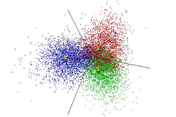
In the old experiment certain words were plotted in the two-dimensional discriminant space as presented in this picture
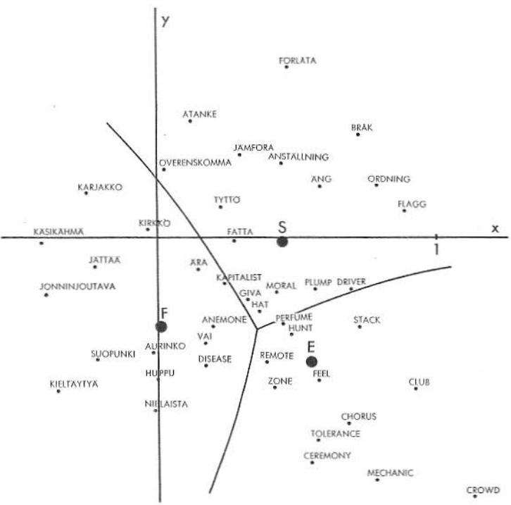
In the latter picture the vertical axis had to be reversed for a proper comparison.
My early (1965) experiment has been described recently (2013) by
Steve Pepper.
This demo in YouTube
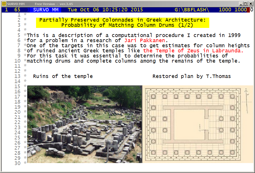
Certain probabilities related to preserved columns of a ruined Temple of Zeus in Lambrounda are obtained by using editorial computing in Survo.
This demo in YouTube
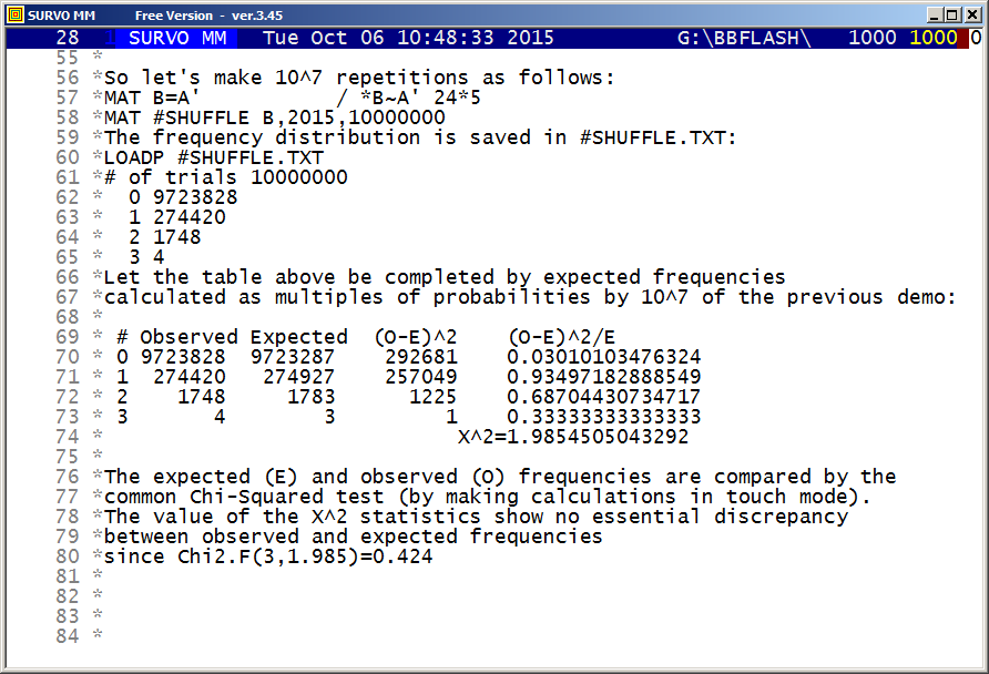
The values of probabilities obtained in the previous demo are compared to empirical frequencies now obtained by simulation.
This demo in YouTube
I was then working as an assistant of Professor Leo Törnqvist and
this practical problem gave us an idea for a more theoretical
problem of deriving the distribution of the distance between
two points chosen uniformly randomly in a metric network.
Törnqvist achieved the result, according to his phenomenal intuitive
thinking, without any formal derivation or proofs.
My task was to formalize the problem, verify the results, and generalize
them. This was done in my
doctoral thesis
in mathematics (1964).
Now I have selected a more practical approach. Due to enormous
progress in computing speed and capacity during 50 years, the
distributions can now be studied by plain simulations giving also more
possibilities for generalizations of the original problem.
Here a simple, regular network G(2) consisting of 2x2 unit squares is
studied for finding the density function of the length of the shortest
path (along the edges) between two random points selected according to
uniform distribution over the entire network of length 12 units.
The results were obtained by using results given in my dissertation.
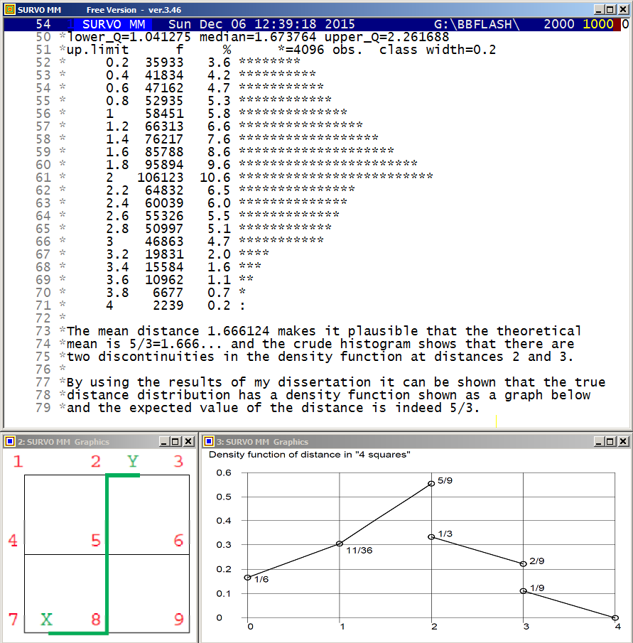
In particular, the expected value of the distance is 5/3=1.666...
In the graph below the theoretical means for networks G(n), n=0,1,2,3,4,
are given
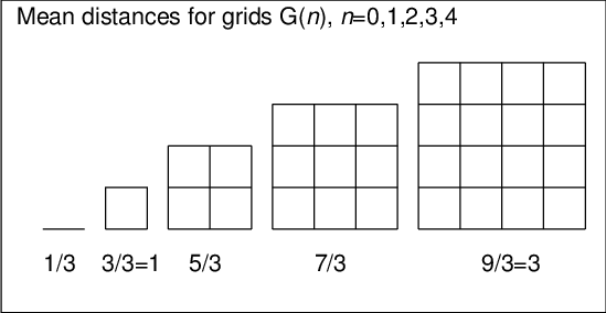
and it is obvious that generally the mean for G(n) is (2n+1)/3. When n grows, this mean divided by n approaches 2/3. This is validated by the fact that it is the expected value of the distance by city metrics between two random points inside a unit square i.e 2 times mean distance in G(0) = 1/3 as explained below.
When we got interested in this topic (in the beginning of 1960ies),
it was natural to start by calculating means for the simplest networks.
like a single edge G(0), or a ring corresponding to G(1).
In the latter case it is easy to see that the first point may be fixed
and thereafter it is seen immediately that the mean is one fourth
of the total length. The fact that for an edge of length 1 the mean is
just 1/3 requires more effort. My favourite (but a little heuristic)
explanation was: "After selecting two random points on the edge,
let's select a third random point. The probability that it falls
between the two earlier ones is 1/3 for symmetrical reasons.
Due to uniformity, the last point covers 1/3 of the total length
'on average'."
This statement can be even generalized: If n random points are selected
from an unit interval, the expected value of the distance of the
extreme points is (n-1)/(n+1). This is 'proved' just in the same way
by selecting once more.
A simple strict proof that for G(0) the mean is 1/3 goes as follows: Let x be he mean. By splitting the unit edge into two equal parts of lenghts 1/2, the probability of selecting the two point on the same half is 1/2 and from different halves also 1/2. The conditional means are 1/2 in the first case and x/2 in the second case. Then we get an equation x=1/2*1/2+1/2*x/2 wherefrom x=1/3. (This was presented by Hannu Väliaho.)
When preparing my PhD thesis I made a program in Elliott Autocode
for the Elliott 803B computer. That program created the exact
density function, but required a lot of computer time.
For example, the G(10) case took about 3 hours.
Now, by using the GDIST operation, approximate results (10^6
simulations) are obtained in less than 10 seconds on my current (2015)
PC. For example, I got the mean 6.995827 which is close enough to
the exact value 7.
The GDIST program calculates shortest distances between any points
on the edges of the network as follows. At first the distance matrix
between all end points is calculated by
Dijkstra's algorithm.
and then, after selecting random points, the various distances through
the end points of the corresponding edges (4 alternatives) are
considered and the minimal distance is selected. As a special case,
the points may be selected on the same edge. Then as the fifth
alternative the distance between the points on that edge must be
considered, too. It should be noted that on 'curved' edges the
last alternative is not necessarily the shortest one.
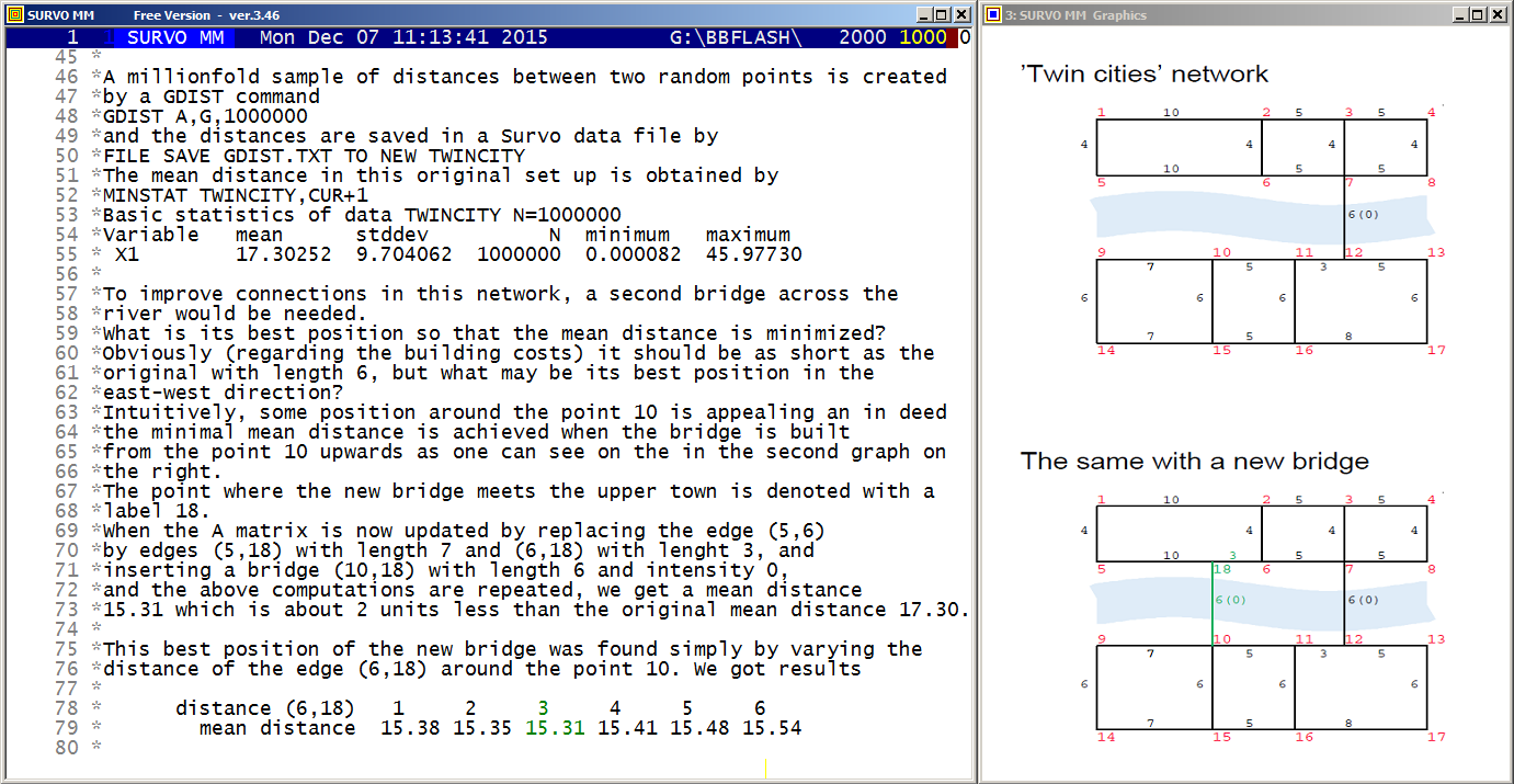
Distance distributions (Twin cities bridge problem)
Distance distributions (n-dimensional cube)
This demo in YouTube
In the A matrix
MAT SAVE AS A
 1  2 10 1
 2  3  5 1
 3  4  5 1
 1  5  4 1
 2  6  4 1
 3  7  4 1
 4  8  4 1
 5  6 10 1
 6  7  5 1
 7  8  5 1
 7 12  6 0
 9 10  7 1
 -  -  - -
Another generalization (not used in this example) is a possibility to add a fifth element (1 or 2) on A-rows implying the edges denoted by 1 as sending regions and edges denoted by 2 as receiving regions so that on traffic between two regions is to be considered.
When applying this possibility to this "twin-cities" so that only traffic between the upper and lower city is studied, in the original situation (no second bridge) the mean distance grows from 17.30 to 24.53 because the internal traffic in the two parts is excluded, but this modification does not change the optimal solution for the additional bridge.
It would be easy make modifications to the GDIST program so that certain gravitation principle is adopted (the probability for taking a journey is dependent on the distace). Obviously this feature can taken into account by a suitable transformation of the density function afterwards.
This demo in YouTube
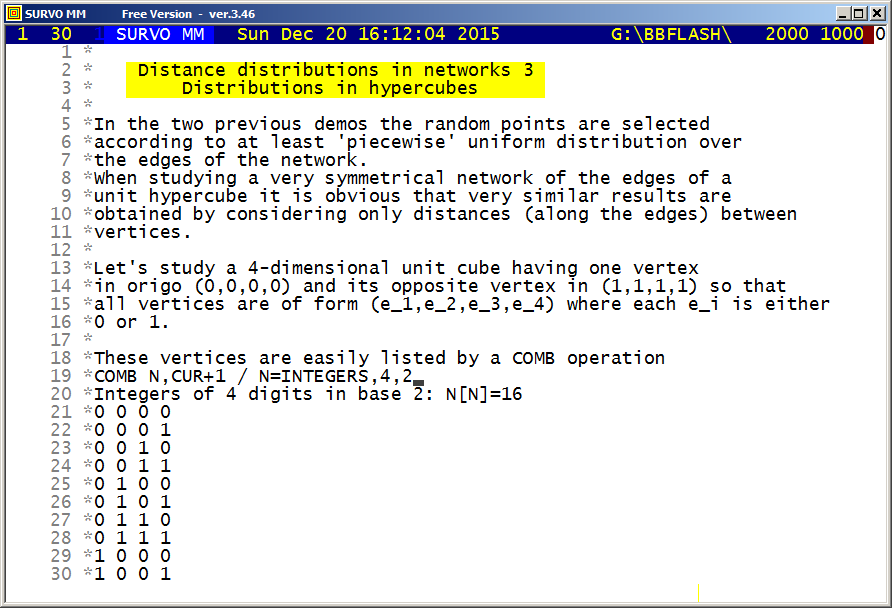
The exact expected value for the distance (along the edges) between
two random points on the edges of the 4-dimensional cube can be computed
as follows:
Because this 'network' is symmetric for each edge, it is sufficient
to assume that the first random point is selected from a given
edge. Each element (vertex, edge, square, cube) of this hypercube
can be denoted by a string of the form abcd where each a,b,c, and d
can be 0, 1, or x, where x covers the range (0,1). Thus for example,
0000 is the first vertex (origo), x000 is the edge from origo to
(1,0,0,0), and xxx0 and x1xx are two of the eight cubes located in the
hypercube.

The mean distances between x000 and the other edges can be
easily computed and they are presented in the following table.

edge mean     edge mean   edge mean   edge mean
x000  1/3     0x00  1     00x0  1     000x  1
x100  5/3     1x00  1     10x0  1     100x  1
x010  5/3     0x10  2     01x0  2     010x  2
x110  8/3     1x10  2     11x0  2     110x  2
x001  5/3     0x01  2     00x1  2     001x  2
x101  8/3     1x01  2     10x1  2     101x  2
x011  8/3     0x11  3     01x1  3     011x  3
x111 11/3     1x11  3     11x1  3     111x  3

The means in the first column are related to 'opposite' edges of
x000. According to terminology used in my dissertation (1964)
they are mirror point sets for x000.
It is clear that mean inside x000 is 1/3, but why the mean
distance between random points on opposite edges is of a unit square
square is 5/3 ?
     .----.
     |    |
     |    |
     .----.
Let it be x. If two random points are selected from the edges of a
unit square, the probablity that they are selected from the same
edge is 1/4, from opposite edges similarly 1/4, and from
neighbouring edges 1/2. The means are 1/3, x, and 1 respectively.
Since the total mean in unit square is 1, we have an equation
   1 = 1/4*1/3 + 1/4*x + 1/2*1
giving x=5/3. The remaining means in the first column are thereafter
easy to comprehend.

The means in the remaining three columns are obvious, since they
are either adjacent to x000 or adjacent through a route of a constant
integer length.

Now the total expected value of the distance in the entire
4-dimensional cube is calculated as

((1*2+3*5+3*8+1*11-1)/3+2*3*(1*1+2*2+1*3))/(4*2^3)=2.03125

The general structure becomes still clearer in the 5-dimensional case
where the expected value has the form

((1*2+4*5+6*8+4*11+1*14-1)/3+2*4*(1*1+3*2+3*3+1*4))/(5*2^4)=2.5291666666667
and 2.5291666666667(12:ratio)=607/240 (0.00000000000003)

On the basis of these expressions it is obvious that
in the n-dimensional case the expression for the mean distance
can be presented in the form

E(n)=((P(n+1)-1)/3+2*(n-1)*Q(n-2))/(n*2^(n-1))

Both P(n) and Q(n) are 'weighted' sums of binomial coefficients.
In fact P-sequence is an inverse binomial transform of an arithmetic
sequence 2,5,8,11,14,... and Q-sequence a similar transform of natural
numbers 1,2,3,4,5,...

The P(n) values for n=2,...,7 are

 n  P(n)
 2  1*2=2
 3  1*2+1*5=7
 4  1*2+2*5+1*8=20
 5  1*2+3*5+3*8+1*11=52
 6  1*2+4*5+6*8+4*11+1*14=128
 7  1*2+5*5+10*8+10*11+5*14+1*17=304

By consulting OEIS (The On-Line Encyclopedia of Integer Sequences)
it is found that the sequence 2,7,20,52,128,304,... is
A066373
and P(n)=(3*n-2)*2^(n-3),  n=2,3,...

The Q(n) values for n=0,1,...,5 are

 n  Q(n)
 0  1*1=1
 1  1*1+2*1=3
 2  1*1+2*2+1*3=8
 3  1*1+3*2+3*3+1*4=20
 4  1*1+4*2+6*3+4*4+1*5=48
 5  1*1+5*2+10*3+10*4+5*5+1*6=112

and OEIS tells that 1,3,8,20,48,112,... is
A001792
and Q(n):=(n+2)*2^(n-1),  n=0,1,...

By substituting expressions of P(n+1) and Q(n-2) into the
the previous formula of E(n) we obtain
E(n)=(((3*n+1)*2^(n-2)-1)/3+2*(n-1)*n*2^(n-3))/(n*2^(n-1))
and this can be simplified into the form
E(n)=n/2+(1-2^(2-n))/(6*n).
This demo in YouTube
This demo in YouTube
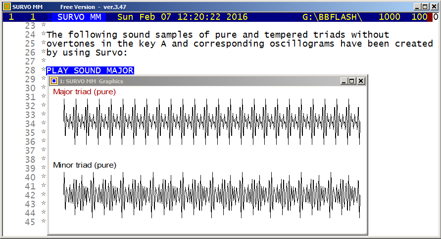
HEADER=[Swiss(20)],Major_triad_(pure)
HOME=0,175 SIZE=649,174
XSCALE=0:_,10*pi:_ YSCALE=[SMALL],-3:_,3:_ pi=3.14159265
X=0,10*pi,pi/60  XDIV=29,600,20  FRAME=0
GPLOT Y(X)=sin(20*X)+sin(25*X)+sin(30*X)
               20:25:30=4:5:6
........................................................
HEADER=[Swiss(20)],Minor_triad_(pure)
HOME=0,0 SIZE=649,174
XSCALE=0:_,10*pi:_ YSCALE=[SMALL],-3:_,3:_ pi=3.14159265
X=0,10*pi,pi/60  XDIV=29,600,20  FRAME=0
GPLOT Y(X)=sin(20*X)+sin(24*X)+sin(30*X)
               20:24:30=10:12:15
........................................................

In the corresponding tempered triads the proportions 20:25:30 and
20:24:30 were replaced by 20:20*2^(4/12):20*2^(7/12) and
20:20*2^(3/12):20*2^(7/12).
At first a Survo data file TEST of 100000 observations for an integer
variable X was created by
FILE MAKE TEST,1,100000,X,2

A fundamental tone of frequency F Hz on sampling rate RATE is described
by a sinus function of the form
S(x):=sin(x*ORDER*2*pi*F/RATE)
where ORDER in the index of an observation in the data file TEST.

When F=440, RATE=44100, and pi=3.141592653589793
S(1) will represent a sample of tone A=440 Hz
and a sample of a pure A Major triad is saved in the data file TEST
as variable X by the VAR operation
VAR X=1000*(S(1)+S(5/4)+S(3/2)) TO TEST
where 1000 gives the sound volume.

Now this TEST file is converted to a WAV file MAJOR.WAV by the Survo
operation
PLAY DATA TEST,X / WAV=MAJOR
and thereafter it can be played as a sound of length
100000/RATE=2.267... seconds by activating
PLAY SOUND MAJOR

The other triads were obtained by replacing S(1)+S(5/4)+S(3/2) in the
VAR operation above by
S(1)+S(6/5)+S(3/2)             pure minor
S(1)+S(2^(4/12))+S(2^(7/12))   tempered major
S(1)+S(2^(3/12))+S(2^(7/12))   tempered minor
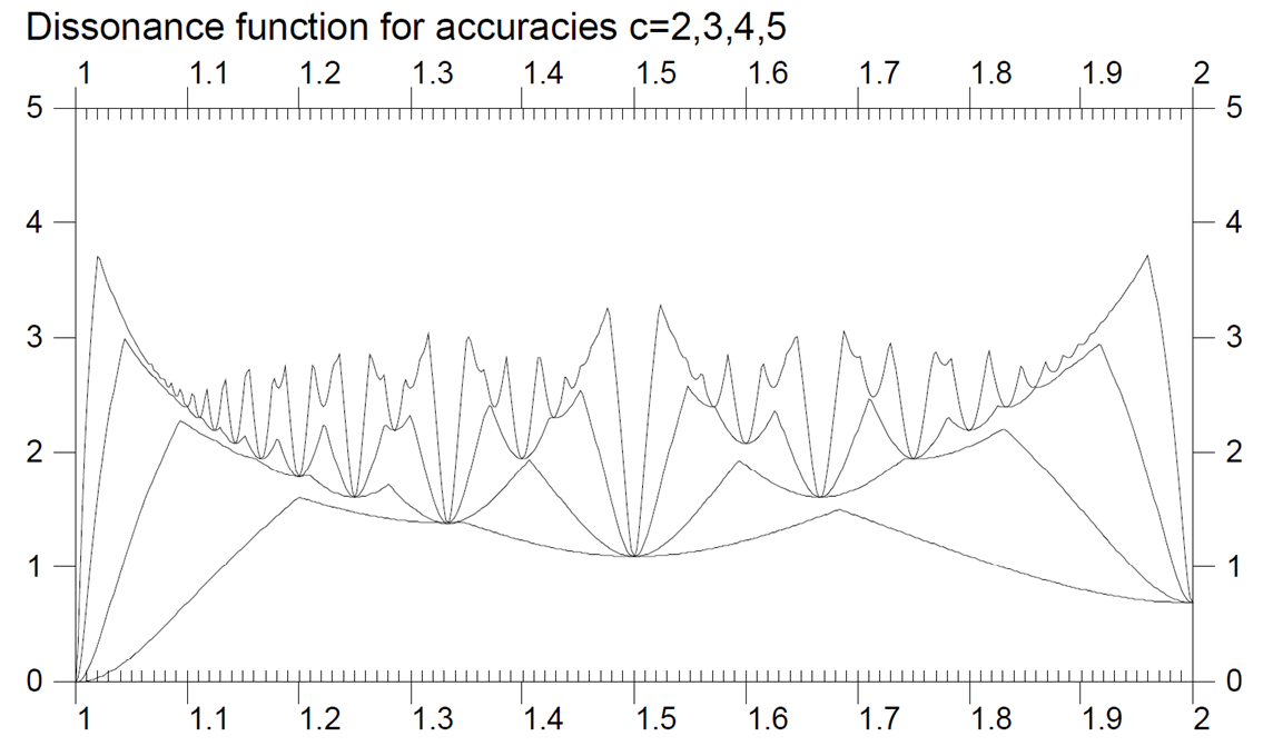
This demo in YouTube
In 1972 when reading the classical treatise "On the Sensations of Tone"
by Helmholtz (1863)
I noticed his
graphical presentation
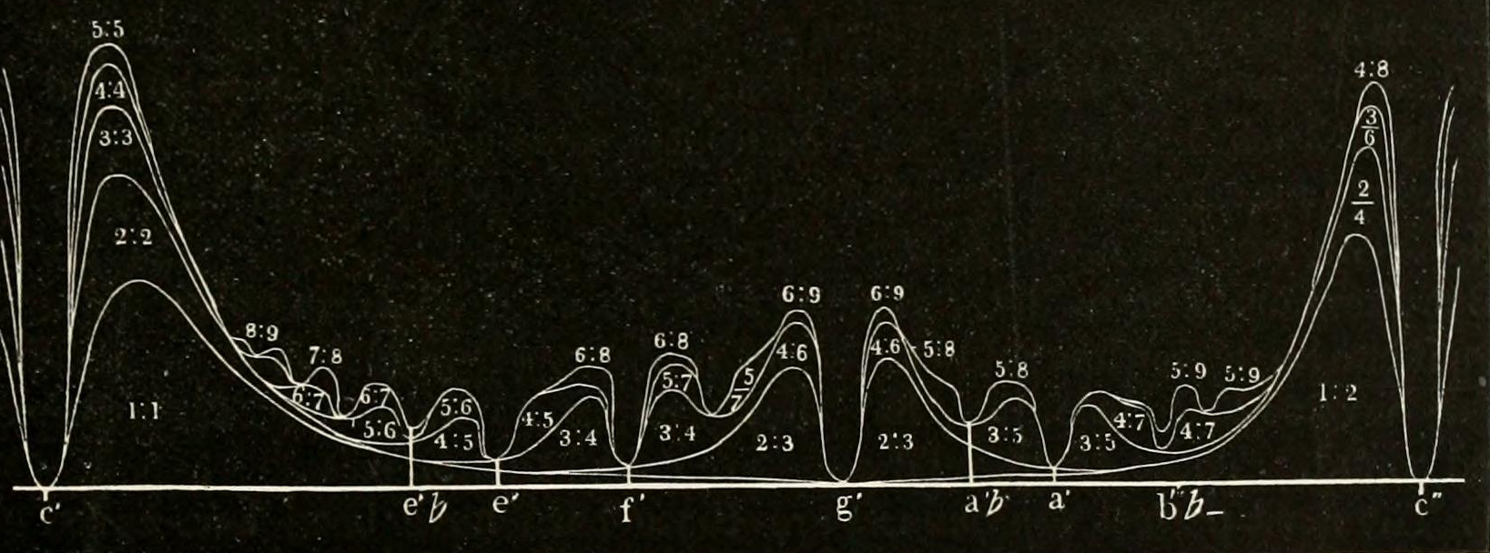
on the consonance of various musical intervals based on practical
experiments on violin.
I formulated these results as a theoretical model as follows:
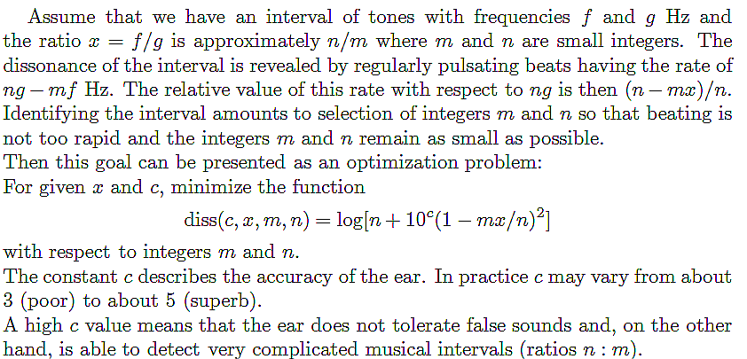
Minimum points of the dissonance function

"Accuracy of the ear"        c=5     c=4     c=3     c=2

Unison                       1:1     1:1     1:1     1:1
Just minor semitone         18:17
Minor diatonic semitone     17:16
Just diatonic semitone      16:15
Septimal diatonic semitone  15:14
Lesser tridecimal 2:3-tone  14:13
Greater tridecimal 2:3-tone 13:12
Neutral second              12:11
Neutral second              11:10
Major second                10:9    10:9
Major second                 9:8     9:8
Septimal major second        8:7     8:7
                            15:13
Septimal major third         7:6     7:6
                            13:11
Just minor third             6:5     6:5     6:5
Neutral third               11:9
Major third                  5:4     5:4     5:4
Diminished major third      14:11
Septimal major third         9:7     9:7
Diminished fourth           13:10
Perfect fourth               4:3     4:3     4:3     4:3
                            15:11
Eleventh harmonic           11:8
Lesser septimal tritone      7:5     7:5
Greater septimal tritone    10:7    10:7
                            13:9
Inversion of 11th harmonic  16:11
Perfect fifth                3:2     3:2     3:2     3:2
                            17:11
Septimal minor sixth        14:9
Undecimal minor sixth       11:7    11:7
Just minor sixth             8:5     8:5
Tridecimal neutral sixth    13:8
Just major sixth             5:3     5:3     5:3
                            17:10
Septimal major sixth        12:7
Harmonic seventh             7:4     7:4     7:4
Small just minor seventh    16:9
Greater just minor seventh   9:5     9:5
Undecimal neutral seventh   11:6    11:6
                            13:7
Just major seventh          15:8
                            17:9
                            19:10
                            21:11
Octave                       2:1     2:1     2:1     2:1
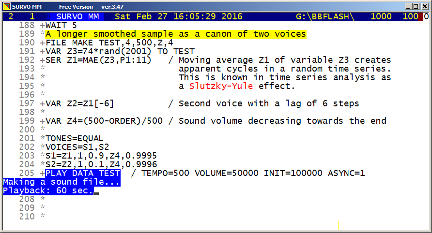
This demo in YouTube
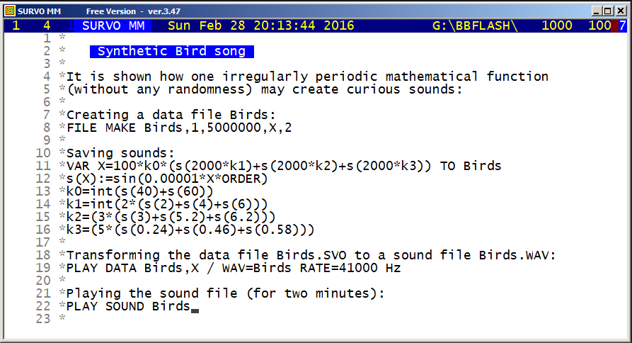
This demo in YouTube
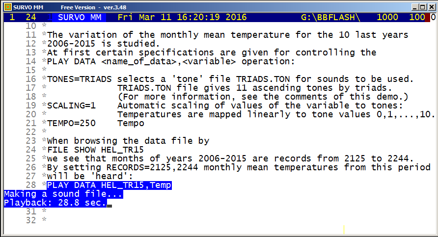
This demo in YouTube
 11 *SAVEP CUR+1,E,TRIADS.TON
 12 *1     / Type
 13 *44100 / Rate Hz
 14 *11    / # of tones
 15 *9     / # of partials
 16 * 0  110   1 S1:.9 S2:.3 S3:.3 S4:.2 S5:.2 S6:.1 S7:.1 S8:.05 S9:.05
 17 * 1  137   1 S1:.9 S2:.3 S3:.3 S4:.2 S5:.2 S6:.1 S7:.1 S8:.05 S9:.05
 18 * 2  165   1 S1:.9 S2:.3 S3:.3 S4:.2 S5:.2 S6:.1 S7:.1 S8:.05 S9:.05
 19 * 3  220   1 S1:.9 S2:.3 S3:.3 S4:.2 S5:.2 S6:.1 S7:.1 S8:.05 S9:.05
 20 * 4  275   1 S1:.9 S2:.3 S3:.3 S4:.2 S5:.2 S6:.1 S7:.1 S8:.05 S9:.05
 21 * 5  330   1 S1:.9 S2:.3 S3:.3 S4:.2 S5:.2 S6:.1 S7:.1 S8:.05 S9:.05
 22 * 6  440   1 S1:.9 S2:.3 S3:.3 S4:.2 S5:.2 S6:.1 S7:.1 S8:.05 S9:.05
 23 * 7  550   1 S1:.9 S2:.3 S3:.3 S4:.2 S5:.2 S6:.1 S7:.1 S8:.05 S9:.05
 24 * 8  660   1 S1:.9 S2:.3 S3:.3 S4:.2 S5:.2 S6:.1 S7:.1 S8:.05 S9:.05
 25 * 9  880   1 S1:.9 S2:.3 S3:.3 S4:.2 S5:.2 S6:.1 S7:.1 S8:.05 S9:.05
 26 *10 1100   1 S1:.9 S2:.3 S3:.3 S4:.2 S5:.2 S6:.1 S7:.1 S8:.05 S9:.05
 27 *
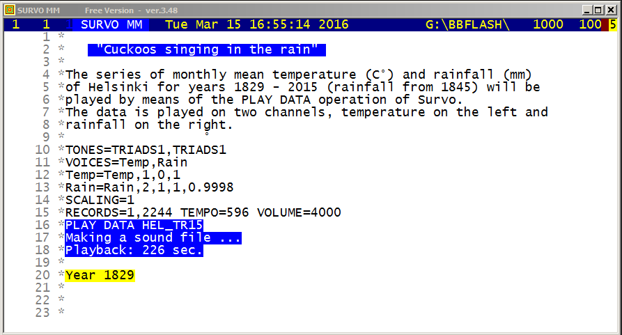
This demo in YouTube
 11 *SAVEP CUR+1,E,TRIADS1.TON
 12 *1     / Type
 13 *44100 / Rate Hz
 14 *11    / # of tones
 15 *3     / # of partials
 16 * 0  110   1 S1:1 S2:0.5 S3:0.25
 17 * 1  137   1 S1:1 S2:0.5 S3:0.25
 18 * 2  165   1 S1:1 S2:0.5 S3:0.25
 19 * 3  220   1 S1:1 S2:0.5 S3:0.25
 20 * 4  275   1 S1:1 S2:0.5 S3:0.25
 21 * 5  330   1 S1:1 S2:0.5 S3:0.25
 22 * 6  440   1 S1:1 S2:0.5 S3:0.25
 23 * 7  550   1 S1:1 S2:0.5 S3:0.25
 24 * 8  660   1 S1:1 S2:0.5 S3:0.25
 25 * 9  880   1 S1:1 S2:0.5 S3:0.25
 26 E10 1100   1 S1:1 S2:0.5 S3:0.25
 27 *
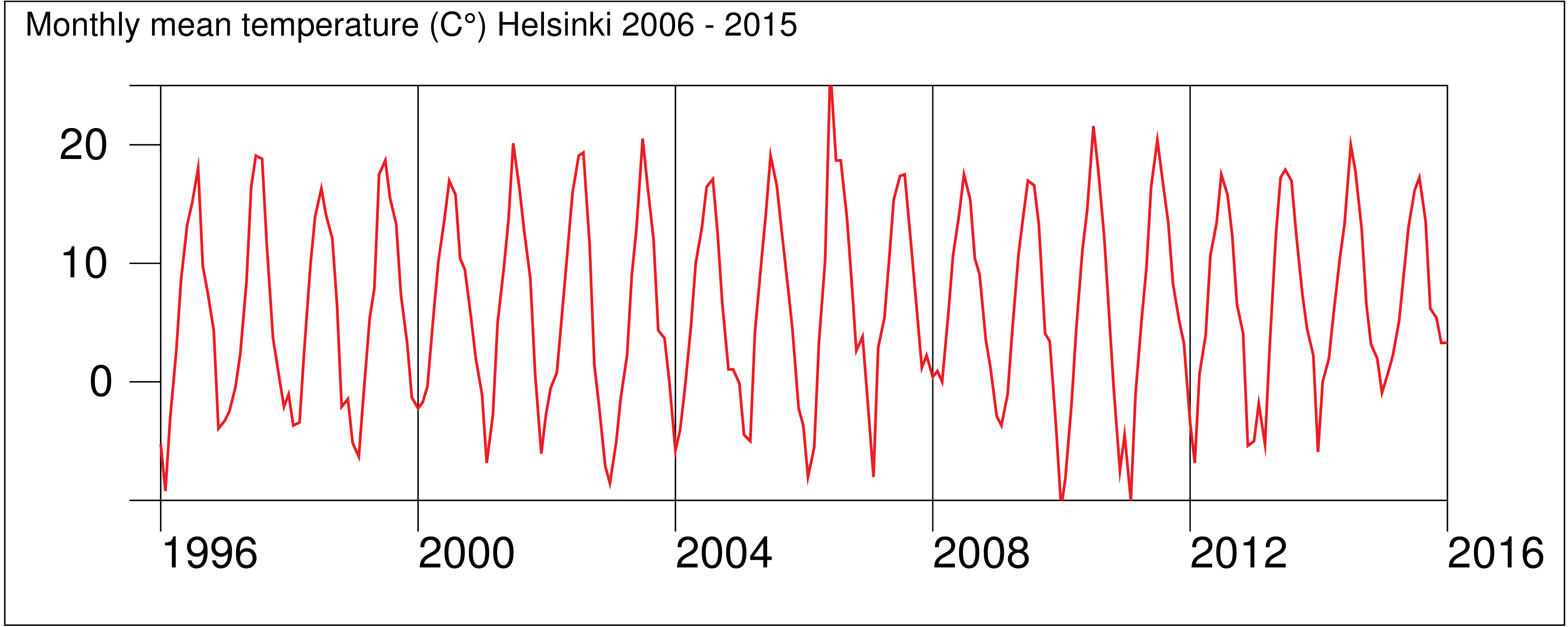
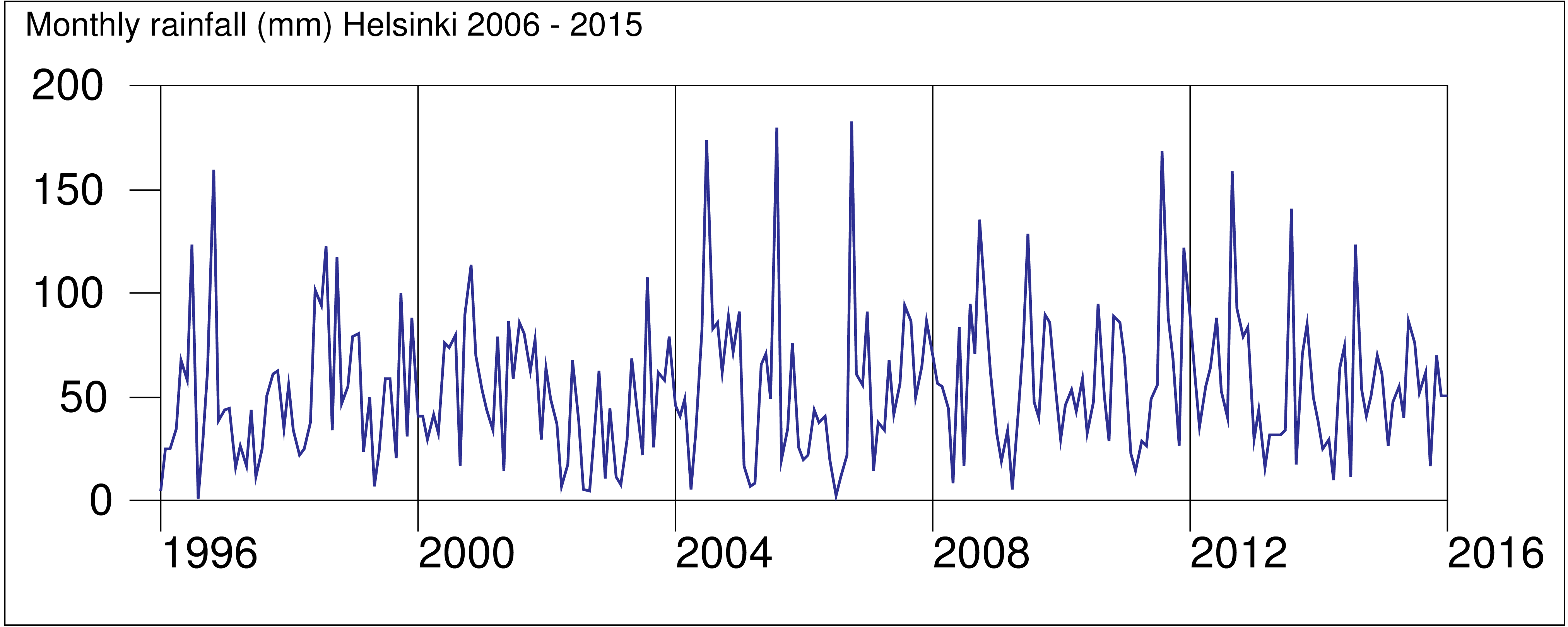
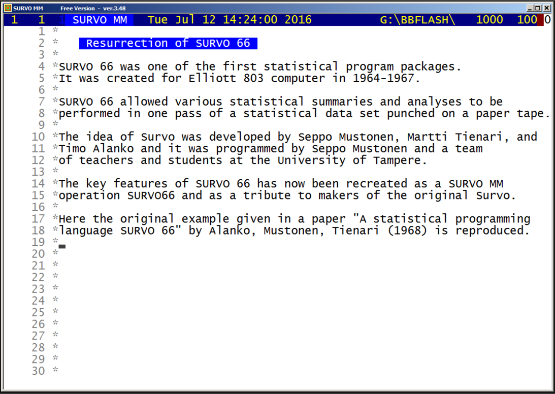
This demo in YouTube
A data set from a statistical research by Dr. Knight on computer
characteristics is used and it has the following contents
as a text file KNIGHT.TXT (N=91):

SHOW KNIGHT.TXT
%
% Date         Scientific      Commercial      Inverse unit
% introduced   power (ops/sec) power (ops/sec) cost (sec/$)
% month year
   4     63     21420.000       9079.000       44.54
   4     65    224374.000     118154.000       15.20
   7     63     67660.000      23420.000       23.98
   4     65      1768.000        990.500      230.90
   1     63     68690.000      58880.000       13.86
   4     65     68497.000      29571.000      103.90
  --     --    ----------     ----------      ------

The main target in this example was to see how well Grosch's law
P=kC^2 fits to Knight's data by using a linear model

ln(P) = a0 + a1*ln(C) + a2*T

where P is 1000 ops/sec, C is $/hour, and T is the age in months.
This law states that a1 should be close to 2.


The program code (with comments in parentheses) is:
SURVO66 KNIGHT.TXT
Evolving Computer performance 1963-1967
M@5                         (number of variables)
CALL@X1 MONTH               (rename variables)
    @X2 YEAR
DEF@MONTH L:1 U:12          (set limits)
   @YEAR L:63 U:67
DIV@SPEED X3 1000           (SPEED=X3/1000)
DIV@COST 3600 X5            (COST=3600/X5)
SUB@Y1 68 YEAR              (Y1=68-YEAR)
MULT@Y2 12 Y1               (Y2=12*Y1)
SUB@AGE Y2 MONTH            (AGE= age in months)
LOG@LSPEED SPEED            (LSPEED=log(SPEED))
   @LCOST COST
CLASS@COSTCL                (classification COSTCL)
      CHEAP 30              (upper limit for CHEAP is 30)
      MODER 90
      EXPNS 500
TABLE@YEAR -                (column variable, default classes 63-67)
      DEVEL COST COSTCL     (table DEVEL, row variable COST with COSTCL)
      T:SPEED               (tables of means and stddevs of SPEED)
CORREL@LSPEED LCOST AGE N:CORR (correlations of variables LSPEEED-AGE)
REGRAN@LSPEED LCOST AGE N:CORR (regression analysis using CORR)
END@

The original names X1,X2,... of the variables are renamed in the code
and the code is activated by the SURVO66 command with the name of
the data set (KNIGHT.TXT) as the only parameter:

The results have been saved in a text file SURVO66.TXT.
They are now loaded into the edit field by
LOADP SURVO66.TXT

Evolving Computer performance 1963-1967

M@5                         (number of variables)
CALL@X1 MONTH               (rename variables)
    @X2 YEAR
DEF@MONTH L:1 U:12          (set limits)
   @YEAR L:63 U:67
DIV@SPEED X3 1000           (SPEED=X3/1000)
DIV@COST 3600 X5            (COST=3600/X5)
SUB@Y1 68 YEAR              (Y1=68-YEAR)
MULT@Y2 12 Y1               (Y2=12*Y1)
SUB@AGE Y2 MONTH            (AGE= age in months)
LOG@LSPEED SPEED            (LSPEED=log(SPEED))
   @LCOST COST
CLASS@COSTCL                (classification COSTCL)
      CHEAP 30              (upper limit for CHEAP is 30)
      MODER 90
      EXPNS 500

TABLE@YEAR -                (column variable, default classes 63-67)
      DEVEL COST COSTCL     (table DEVEL, row variable COST with COSTCL)
      T:SPEED               (tables of means and stddevs of SPEED)

Table: DEVEL
Column variable: YEAR
Row    variable: COST
Frequencies
               63       64       65       66       67    Total
   CHEAP        6        4       10        7        4       31
   MODER        7       11        9        5        1       33
   EXPNS        6        6        6        6        3       27
   Total       19       21       25       18        8       91
Chi2=6.0617 df=8 P=0.64032

Means of SPEED
               63       64       65       66       67    Total
   CHEAP 5.529187 2.078415 20.80887 1.658377 36.56175 13.14300
   MODER 13.25171 54.88778 50.50800 439.0866 154.8420 106.1023
   EXPNS 198.3025 1371.591 1123.889 1875.849 1419.726 1173.221
   Total 69.25011 421.0299 296.2399 747.8964 570.0332 391.0525

Standard deviations of SPEED
               63       64       65       66       67    Total
   CHEAP 9.650197 2.826062 28.63729 2.051873 55.15149 26.80980
   MODER 15.16012 59.95012 47.31911 484.0829        - 231.6778
   EXPNS 170.9234 2770.993 1412.064 2187.189 1567.665 1823.350
   Total 127.8364 1517.006 801.2234 1472.591 1095.507 1114.315

CORREL@LSPEED LCOST AGE N:CORR (correlations of variables LSPEEED-AGE)
Means and standard deviations
MATRIX CORR_M.M
S66MSN
///          Mean   Stddev        N
LSPEED    3.05430  3.11669 91.00000
LCOST     3.90558  1.23418 91.00000
AGE      32.97802 14.36120 91.00000
Correlation coefficients
MATRIX CORR_R.M
S66CORR
///        LSPEED    LCOST      AGE
LSPEED    1.00000  0.80688 -0.17920
LCOST     0.80688  1.00000  0.05398
AGE      -0.17920  0.05398  1.00000

REGRAN@LSPEED LCOST AGE N:CORR (regression analysis using CORR)
LINREG S66DATA>.M,CUR+1 / RESULTS=0
Linear regression analysis: Data S66DATA>.M, Regressand LSPEED    N=91
Variable Regr.coeff.    Std.dev.    t     beta
AGE      -0.048483       0.012672 -3.826 -0.223
LCOST     2.068079       0.147458  14.02  0.819
constant -3.423891       0.716240 -4.780
Variance of regressand LSPEED=9.713751390 df=90
Residual variance=2.972162239 df=88
R=0.8372 R^2=0.7008

END@

Grosch's law seems to fit well to Knight's data.
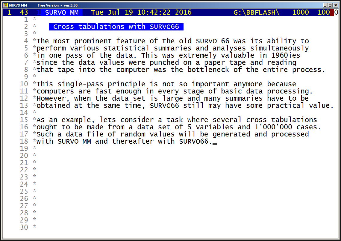
This demo in YouTube
It is shown that SURVO66 is essentially faster than the TAB
operation of SURVO MM when many cross tabulations should be done
from a large data set.
See also Resurrection of SURVO 66
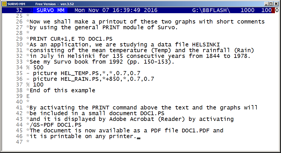
This demo in YouTube
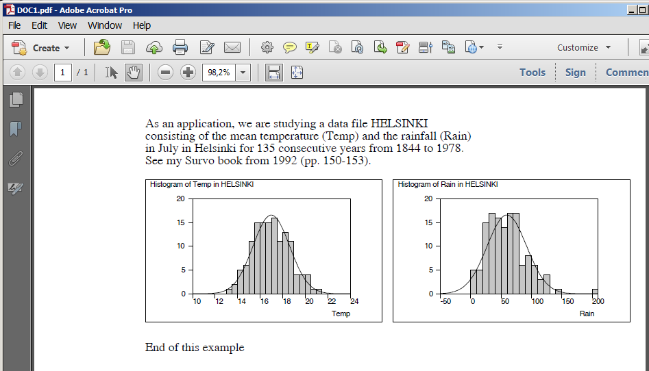
- [ArialB(11)][line_spacing(14)]next after the PRINT line in the previous example, the result will be
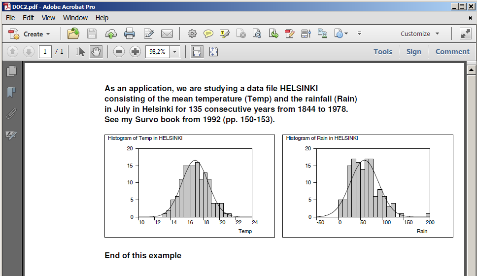

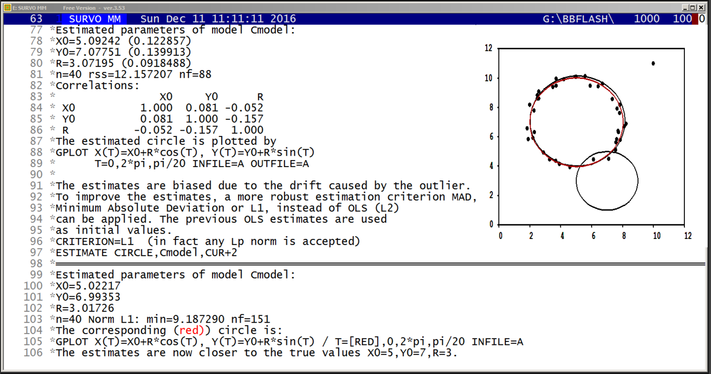
This demo in YouTube
DATA CIRCLE
  X    Y
 30   68
 50   -6
110  -20
 35   15
 45   97

MODEL Cmodel
sqrt((X-X0)^2+(Y-Y0)^2)=R

ESTIMATE CIRCLE,Cmodel,CUR+1
Estimated parameters of model Cmodel:
X0=96.0759 (1.69426)
Y0=48.1352 (1.11286)
R=69.9602 (1.33064)
n=5 rss=3.126753 nf=120
Correlations:
                X0     Y0      R
 X0          1.000  0.611  0.892
 Y0          0.611  1.000  0.675
 R           0.892  0.675  1.000
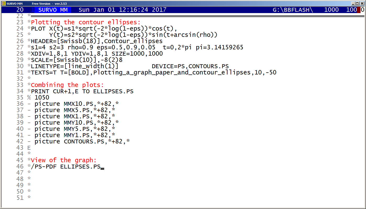
This demo in YouTube
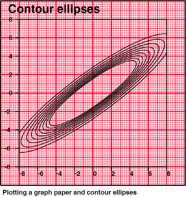
The first version of this graph was given on page 40 of
my document about SURVO 84
in 1984 and indicates that I had found the formulas
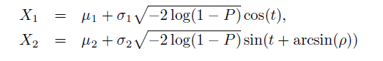
for contour ellipses on the confidence level P
of a general bivariate normal distribution
as well as the generalized
Box-Müller formulas
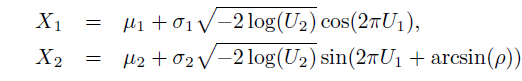
for generating observations of a general bivariate normal distiribution
with a correlation coefficient ρ from two independent Uniform(0,1) variables
already then and thus earlier than told in my document
Two formulas related to two-dimensional normal distribution.
*Originally
arcsin(ρ) had to be replaced by arctan(ρ/(sqrt(1-ρ*ρ))
since arctan was the only inverse trigonometric funtion available in SURVO 84.
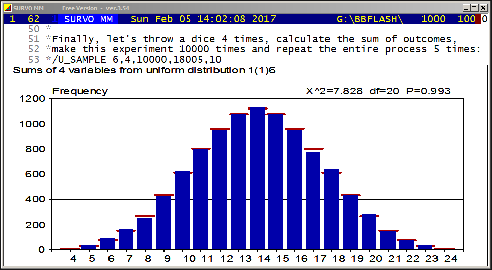
This demo in YouTube
Samples from distributions related to the discrete uniform
distribution are shown as dynamic histograms generated step by step.
In fact, these graphs are scatter plots of data sets of two variables.
The X variable is a discrete random variate and the values of the Y
variable are cumulative frequencies of distinct X values.
This setup is generated, for example, for discrete uniform variable
with values 1,2,3,4,5,6 by MAT commands
MAT A=ZER(n,1) / n is the sample size
MAT #TRANSFORM A BY int(6*rand(2017)+1)
MAT B=ZER(n,2)
MAT B(1,1)=A
MAT #CUMFREQ(B)
where the last command computes the cumulative sums of distinct values in the first column as elements of the second column.
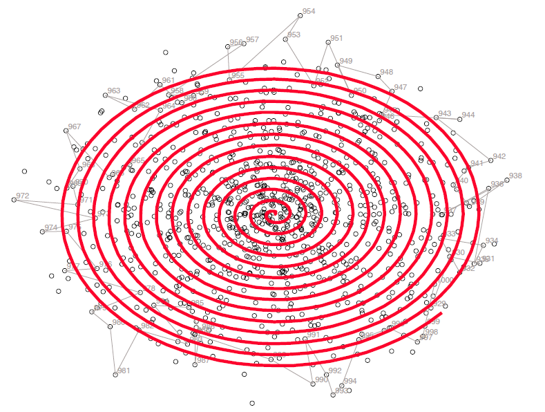
This demo in YouTube
In 1970s it was possible to create Survo graphics by the
Wang 2272 digital drum plotter
connected to a
Wang 2200 minicomputer.
This advantage was lost when plotters were replaced laser printers or graphic screens. On a laser printer, the entire plotting process takes place out of sight. On the screen everything happens too quickly.
The main target of this demo is to point out that there may be cases where it is meaningful to slow down the plotting process (by using the SLOW specification) so that the user is able to see potential interactions between observations and/or variables.
Other examples of slow plotting in Survo are given in
Sampling from a discrete uniform distribution.
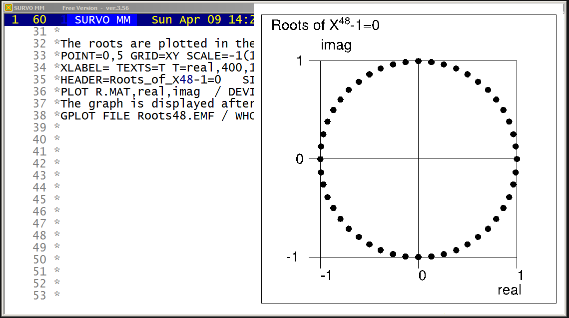
This demo in YouTube
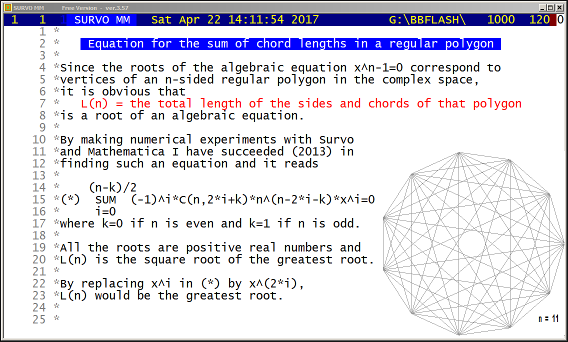
This demo in YouTube
For example, equations C11*E11=R11 (divided by 2*11) lead to formulas

sin(5π/11)+sin(4π/11)+sin(3π/11)+sin(2π/11)+sin(1π/11) = cot(1π/22)/2
sin(5π/11)-sin(4π/11)+sin(3π/11)+sin(2π/11)-sin(1π/11) = cot(3π/22)/2
sin(5π/11)-sin(4π/11)+sin(3π/11)-sin(2π/11)+sin(1π/11) = cot(5π/22)/2
sin(5π/11)+sin(4π/11)-sin(3π/11)-sin(2π/11)-sin(1π/11) = cot(7π/22)/2
sin(5π/11)-sin(4π/11)-sin(3π/11)+sin(2π/11)+sin(1π/11) = cot(9π/22)/2

and equations C15*E15=R15 (divided by 2*15) to formulas

 sin(7π/15)+sin(6π/15)+sin(5π/15)+sin(4π/15)+sin(3π/15)+sin(2π/15)+sin(1π/15) = cot(1π/30)/2
            sin(6π/15)                      +sin(3π/15)                       = cot(3π/30)/2
                       sin(5π/15)                                             = cot(5π/30)/2
 sin(7π/15)-sin(6π/15)+sin(5π/15)-sin(4π/15)+sin(3π/15)-sin(2π/15)+sin(1π/15) = cot(7π/30)/2
            sin(6π/15)                      -sin(3π/15)                       = cot(9π/30)/2
-sin(7π/15)+sin(6π/15)-sin(5π/15)+sin(4π/15)+sin(3π/15)-sin(2π/15)+sin(1π/15) = cot(11π/30)/2
-sin(7π/15)+sin(6π/15)+sin(5π/15)-sin(4π/15)-sin(3π/15)+sin(2π/15)+sin(1π/15) = cot(13π/30)/2

The elements of the vector En are lengths of edges and chords
(multiplied by n)
e_i = 2*sin(((n+1)/2-i)π/n), i=1,2,...,(n-1)/2
for odd n and
e_i = 2*sin((n/2+1-i)π/n), i=1,2,...,n/2
for even n.
In the latter case e_1=2 is replaced by e_1=1.

The elements of the vector Rn are
r_i = n*cot((2*i-1)π/(2n)), i=1,2,...,⌊n/2⌋
and found originally as the square roots of the roots of
equation

 (n-k)/2
   Σ    (-1)^i*C(n,2*i+k)*n^(n-2*i-k)*x^i=0
  i=0

where k=0 if n is even and k=1 if k is odd.


The essential tools for finding the Cn matrices are the
MAT #ARFIND and MAT #SPREAD commands of SURVO MM.

MAT #ARFIND,n,A
finds the Cn coefficients for 'roots' unique for n as linear
combinations of chord lengths with coefficients +1,-1.
The general setup related to n is saved as a matrix
file A.MAT and the coefficients of the linear combinations in
a matrix file Cn.MAT.

According to my conjecture the valid coefficients related to
row i of Cn (in a 'unique' case) are to be selected from

 c_ij=±sgn(cos(q_ni*pi*(2*j-k)/(2*i-1)))), i,j=1,,2,...,⌊n/2⌋

where k=1 for odd n and k=2 for even n and q_ni is a positive integer.

The correct value of q_ni is selected from alternatives
q_ni=1,2,...,⌊(n/2)⌋
so that the linear combination of chord lengths with coefficients
c_ij gives the i'th 'root'.
The selected q value and its sign coefficient appear as two first
columns of A.MAT.

Then according to this conjecture the correct coefficients are
found in n/4 trials on average. Without relying to this
conjecture, about 2^(n-2) alternatives should be tested
which is an essentially harder task.

The indefined rows of Cn (related to factors of n) remain filled with
zeroes and the origin of these rows is revealed by the 'factor' and
'index' columns of the matrix A.

The details of MAT #ARFIND can be found in its current C code.

By creating C matrices for factors given in matrix A by
repeated applications of MAT #ARFIND, the 'empty' rows in the
original Cn matrix can be filled by the MAT #SPREAD operation.


Table of q_ni coefficients

By defining for positive integers n,k, n>=k

                     mod(n,k) if mod(n,k)<=⌊k/2⌋
        amod(n,k) =
                     k - mod(n,k) otherwise

I have concluded experimentally that q_ni values depend on n only
through m=amod(n,i) values. Then it has been possible to create a table
of q values of the following form

 i/m    1  2  3  4  5  6  7  8  9 10 11 12 13 14 15 16 17 18 19 20 21
 2      1  .  .  .  .  .  .  .  .  .  .  .  .  .  .  .  .  .  .  .  .
 3      2  1  .  .  .  .  .  .  .  .  .  .  .  .  .  .  .  .  .  .  .
 4      3  2  1  .  .  .  .  .  .  .  .  .  .  .  .  .  .  .  .  .  .
 5      4  2 *3  1  .  .  .  .  .  .  .  .  .  .  .  .  .  .  .  .  .
 6      5  3  2  4  1  .  .  .  .  .  .  .  .  .  .  .  .  .  .  .  .
 7      6  3  2  5  4  1  .  .  .  .  .  .  .  .  .  .  .  .  .  .  .
 8      7  4 *3  2 *5 *6  1  .  .  .  .  .  .  .  .  .  .  .  .  .  .
 9      8  4  3  2  5  7  6  1  .  .  .  .  .  .  .  .  .  .  .  .  .
10      9  5  3  7  2  8  4  6  1  .  .  .  .  .  .  .  .  .  .  .  .
11     10  5 *3  8  2 *6 *7  4 *9  1  .  .  .  .  .  .  .  .  .  .  .
12     11  6  4  3  7  2  5 10  9  8  1  .  .  .  .  .  .  .  .  .  .
13     12  6  4  3 *5  2  9 11  7*10  8  1  .  .  .  .  .  .  .  .  .
14     13  7 *3 10  8 *6  2  5 *9  4 11*12  1  .  .  .  .  .  .  .  .
15     14  7  5 11  3 12  2  9  8 13  4  6 10  1  .  .  .  .  .  .  .
16     15  8  5  4  3 13 11  2 12 14  7  9  6 10  1  .  .  .  .  .  .
17     16  8 *3  4 10 *6  7  2 *9  5*11*12 14 13*15  1  .  .  .  .  .
18     17  9  6 13 *5  3 *7 11  2*10  8 16  4*14*15 12  1  .  .  .  .
19     18  9  6 14 11  3  8  7  2 13  5 17 10  4 16 15 12  1  .  .  .
20     19 10 *3  5  4 *6 14 17 *9  2 16*12*13  7*15 11  8*18  1  .  .
21     20 10  7  5  4 17  3 18 16  2 13 12 11 19 15  9  6  8 14  1  .
22     21 11  7 16 13 18  3  8 12 15  2  9  5 20 10  4 19  6 17 14  1

The row i in the table is a permutation of integers 1,2,...,i-1.
The numbers preceded by *'s (being the same as column numbers)
extend the row i to a permutation, but cannot appear as amod() values
due to common factors with 2*i-1. Let's call them dummy values.
The column 'q' in the A matrix obtained by MAT #ARFIND,n,A gives
the pertinent q_ni values and the table may be extended by using
them.
The same table extended to row 75
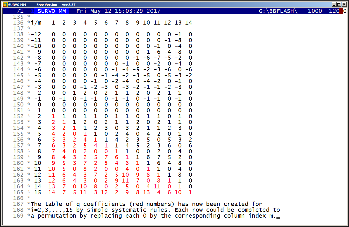
This demo in YouTube
Already in 2013 I tried to find an algorithm for computing the table of the q_ni numbers appearing in the coefficients c_ij=±sgn(cos(q_ni*pi*(2*j-k)/(2*i-1)))), i,j=1,,2,...,⌊n/2⌋ of the linear combinations needed in the previous demo. When noticing that the row i of the table of q's is a permutation of integers 1,2,...,i-1, it was natural to search for a direct rule of selecting the right permutations and maybe that it is still possible. For example, it is temptating to think that the rows could be related to residues (mod i) of some functions of i. I have not found such a direct formula. It is surprising that now an extension of the table by simple arithmetical tricks leads to these permutations and thus we seem to have an 'algorithmic formula'. The q_ni values depend on n only through m=amod(n,i) values as told in the previous demo. If the sequence of integers in the column m of the table of q's is denoted by q(i,m), i=1,2,..., the recursive relation q(i,m)=2*q(i-m,m)-q(i-2*m,m), i=1,2,... seems to be generally valid and the table of q's can be completed in the following way by using that recursion (and readily available permutations until i=43):It is crucial to see that the row i (i=2,3,...) starting by a specific permutation of numbers 1,2,...,i-1 (in red) is followed by the same numbers in reversed order (in green), then followed by one dummy value and thereafter this scheme is repeated 'forever'. Dummies may also appear in permutations (typically as multiples of the 'correct' number) but it is not harmful since they cannot appear as q coefficients. For simplicity, dummies can be replaced by 0's. It is also essential to notice that any column can be continued upwards by a still simpler recursion so that q(-i,m)=-q(i+1,m) i=0,1,2,... after setting plain 0's to the row 1. For example, for m=4 we have i ... -4 -3 -2 -1 0 1 2 3 4 5 ... q(i,4) ... -1 -1 -2 -1 0 0 1 2 1 1 ... Then it is obvious that the table of q's can be generated simply row by row using the recursive relation. For example, assume that we have rows down to 5 ready with upward 'mirror' completions for 5 first columns: i/m 1 2 3 4 5 6 7 8 9 10 11 12 13 14 15 16 17 18 19 20 21 -5 -4 -4 -2 0 -1 -1! -3 -3 -2 -1 -1 -2 -2 -2 -1 -1 -2! 0 -1 -1 -1 0 -1 -1 0 0 0 0! 0 0 1 0 0 0 0 0! 0 0 0 0 0 0 0 0 0 0 0 0 0 0 0 0 2 1 1! 0 1! 1 0 1 1 0 1 1 0 1 1 0 1 1 0 1 1 0 3 2 1 1! 2 0 2 1 1 2 0 2 1 1 2 0 2 1 1 2 0 2 4 3! 2! 1 1 2 3 0 3 2 1 1 2 3 0 3 2 1 1 2 3 0 5 4! 2 0 1 1 0 2 4 0 4 2 0 1 1 15 2 4 0 4 2 0 Then the start of the next row emerges for the 5 first elements recursively as (!'s after numbers used in recursion) 6 5 3 2 4 1 giving the permutation and the row is completed by the rule told above: 6 5 3 2 4 1 1 4 2 3 5 0 5 3 2 4 1 1 4 2 3 5 On basis of these findings it was possible to create an essentiallly faster algorithm for computing the Cn matrices demonstrated here. This new algorithm is now available in SURVO MM as MAT #QFIND(n) operation and computing the table of q numbers is at least ten times faster than before. The MAT #ARFIND operation is replaced by MAT #QRFIND operation working like MAT #ARFIND but does the job much faster by using a readily computed large table of q values. By using MAT #QRFIND I have computed the linear combinations (with coefficients ±1) for the roots of the equation (presented in the preceding demo) for all prime numbers n less than 10000. At the same time I have checked that coefficients really are either +1 or -1 and linear combinations give the true roots. It has also been verified that each row i in the table of q's gives a permutation of numbers 1,2,...,i-1 (when each possible 0 is replaced by the column index m) and each permutation is of order 2 with i-1 as its first element and 1 as the last one. Although the table of q's was computed only once in this experiment, and it takes a few seconds, the entire checking process lasted on my current PC about 15 hours (a lot of matrix manipulations).
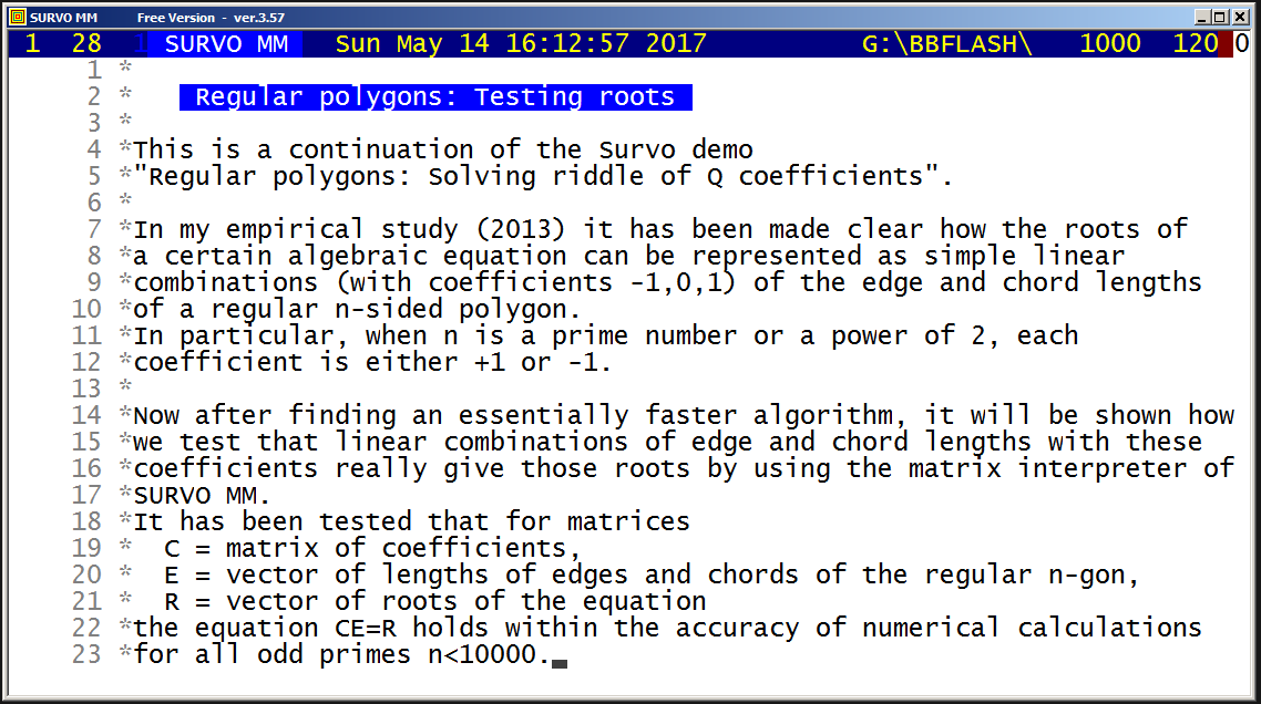
This demo in YouTube
10 *
11 *TUTSAVE C_TEST
12 / def Wn=W1 Wdivisor=W2 Wremainder=W3 Wsquare=W4 Wt=W5 Wt2=W6
13 *{tempo 1}{R}
14 /
15 *{ref set 1}
16 + S: n={print Wn} m=({print Wn}-1)/2{R}
17 *MAT #QRFIND {print Wn},Q5000.TXT,A{act}{R}
18 / Testing that coefficients Cn are 1 or -1
19 *MAT A=C{print Wn}{act}{R}
20 *MAT TRANSFORM A BY abs(X#){act}{R}
21 *MAT B=CON(m,m){act}{R}
22 *MAT A=A-B{act}{R}
23 *MAT TRANSFORM A BY abs(X#){act}{R}
24 *MAT A=SUM(SUM(A)'){R}
25 *MAT_A(1,1)={act}{l} {save word Wt}{R}
26 /
27 *MAT R=ZER(m,1){act} pi=3.141592653589793{R}
28 *MAT E=R{act}{R}
29 *MAT TRANSFORM R BY cot((2*I#-1)*pi/(2*n)){act}{R}
30 *MAT TRANSFORM E BY 2*sin(((n+1)/2-I#)*pi/n){act}{R}
31 *MAT A=MTM(C{print Wn}*E-R){act}{R}
32 *MAT_A(1,1)={act}{l} {save word Wt2}{R}
33 *COPY CUR+1,CUR+1 TO C_TEST.TXT{R}
34 *{erase}{print Wn} {print Wt} {print Wt2}{home}{u}{act}
35 / Next prime number
36 + A: {Wn=Wn+2}{Wdivisor=1}
37 + B: {Wdivisor=Wdivisor+2}{Wremainder=Wn%Wdivisor}
38 - if Wremainder = 0 then goto A
39 *{Wsquare=Wdivisor*Wdivisor}
40 - if Wsquare < Wn then goto B
41 *{ref jump 1}{goto S}{end}
42 *
   3 0 4.9303806576313e-032
   5 0 2.0954117794933e-031
   7 0 6.1629758220392e-032
  11 0 3.5745259767827e-031
  13 0 3.4266145570538e-030
  17 0 2.3611901118188e-030
  19 0 5.3810482646179e-030
  23 0 1.4687141755897e-029
  29 0 1.4881468087286e-029
....
9931 0 2.5192799756962e-022
9941 0 1.2926419087749e-022
9949 0 6.8344417909304e-022
9967 0 1.2351984585185e-022
9973 0 5.3219957169430e-022
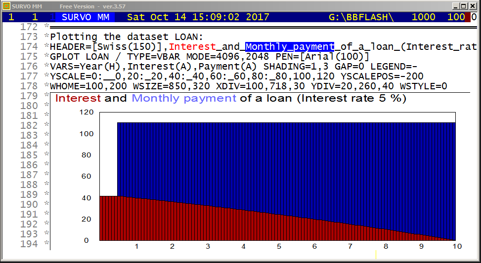
This demo in YouTube
*
*    Loan calculator for fixed monthly payments
*
*Assume that the loan amount is K (euros), the yearly interest rate is P
*(per cent) and the loan term is T years (n=12*T months).
*The loan will be paid monthly by a constant sum x consisting of both
*the interest and amortization.
*It will be described how the monthly payment is divided into those
*two components during the entire loan period.
*Lets denote p=P/12/100 and q=1/(1+p) and thus q is the monthly discount
*factor. Then the monthly payment x is determined by requiring that
*the sum of the discounted payments must be equal to the original loan
*amount K and thus
*   K = x*q + x*q^2 + ... + x*q^n = x*q*[1 + q + q^2 + ... + q^(n-1)]
*                                 = x*q*(1-q^n)/(1-q)
*giving
*   x = K/q/(1-q^n)*(1-q).
*If during the v first months mere payment of the interest is permitted,
*the monthly payment will be
*   x = K/q/(1-q^(n-v))*(1-q)
*since the loan will be shortened only during the last n-v months.
*
*
*Lets study a case K=10000, P=5, T=10, v=6 and recall the notations
*n=12*T p=P/12/100 q=1/(1+p) .
*Our aim is to create a table with columns
*  Time     Interest     Payment         Remaining
*as a Survo data set LOAN.
*
*The columns of the table are calculated by the VAR commands
*VAR Time=ORDER TO LOAN  / Time in months 1-120
*
*Monthly=K/q/(1-q^(n-v))*(1-q) / Monthly payment (x above)
*
*Interest=if(Time<=v)then(K*p)else(Remaining[-1]*p)
*Remaining=if(Time<=v)then(K)else(Remaining[-1]-Payment)
*Payment=if(Time<=v)then(0)else(Monthly-Interest)
*VAR Interest,Payment,Remaining TO LOAN
*
*DATA LOAN,A,A+119,N,M
M  1234   1234.1234567  1234.1234567   1234567.1234567
N  Time     Interest     Payment         Remaining
A     1     41.6666667     0.0000000     10000.0000000
*     2     41.6666667     0.0000000     10000.0000000
*     3     41.6666667     0.0000000     10000.0000000
*     4     41.6666667     0.0000000     10000.0000000
*     5     41.6666667     0.0000000     10000.0000000
*     6     41.6666667     0.0000000     10000.0000000
*     7     41.6666667    68.7083351      9931.2916649
*     8     41.3803819    68.9946198      9862.2970451
*     9     41.0929044    69.2820974      9793.0149477
*    10     40.8042289    69.5707728      9723.4441749
*    11     40.5143507    69.8606510      9653.5835239
*    12     40.2232647    70.1517371      9583.4317868
*    13     39.9309658    70.4440360      9512.9877508
*    14     39.6374490    70.7375528      9442.2501980
*    15     39.3427092    71.0322926      9371.2179054
*   ---     ----------   -----------      ------------
*   115      2.7195771   107.6554247       545.0430849
*   116      2.2710129   108.1039889       436.9390960
*   117      1.8205796   108.5544222       328.3846738
*   118      1.3682695   109.0067323       219.3779415
*   119      0.9140748   109.4609270       109.9170145
*   120      0.4579876   109.9170142         0.0000003
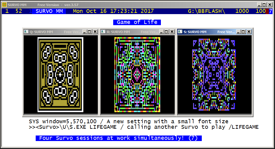
This demo in YouTube
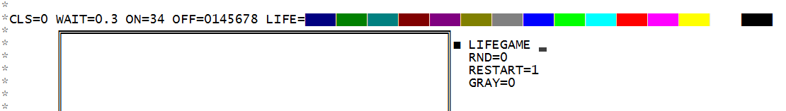
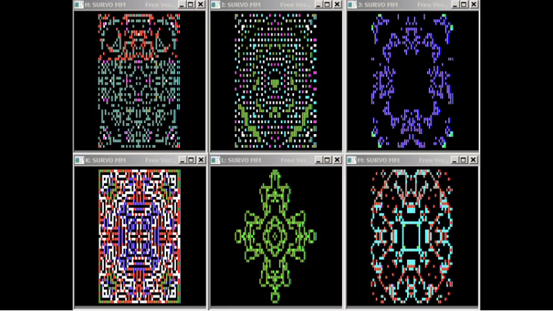
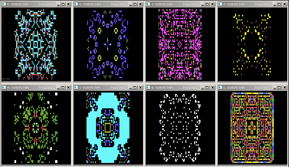
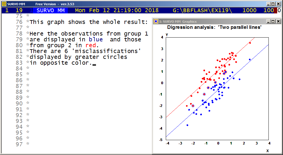
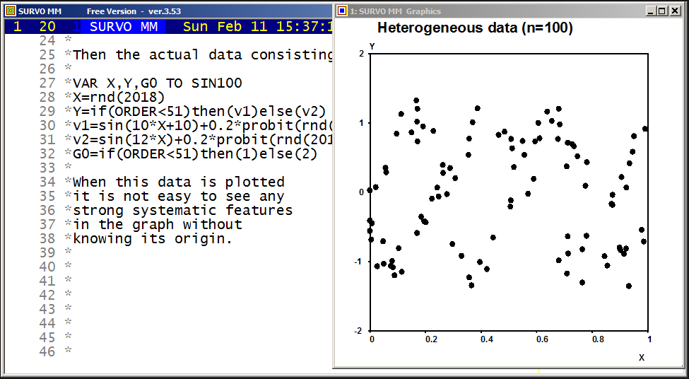
This demo in YouTube
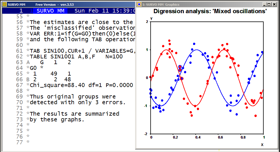
*Now the model is defined as
*MODEL M
*Y=sin(A*X+B) or Y=sin(C*X+D)
*
*and starting from 'poor' initial values
*A=8 B=12 C=15 D=0
*The DIGRES operation gives the results
*
*DIGRES SIN100,M,CUR+1
*Estimated parameters of model M:
*A=9.82352
*B=10.1049
*C=12.2938
*D=-0.154894
*n=100 rss=4.017864 R^2=0.93380 nf=671
*
*The estimates are close to the true values 10,10,12,0.
*
*
*MODEL M1
*Y=sin(A*X+B)
*
*MASK=AA--A--
*A=10 B=10 RESULTS=0
*ESTIMATE SIN100,M1,CUR+1 / IND=G,1 First group
*Estimated parameters of model M1:
*A=9.82352 (0.11347)
*B=10.1049 (0.0657281)
*n=51 rss=1.653080 R^2=0.93311 nf=39
*
*MODEL M2
*Y=sin(C*X+D)
*MASK=AA--A--
*
*C=12 D=0
*ESTIMATE SIN100,M2,CUR+1 / IND=G,2 Second group
*Estimated parameters of model M2:
*C=12.2938 (0.161625)
*D=-0.154893 (0.0904904)
*n=49 rss=2.364784 R^2=0.92972 nf=33
*
The estimated parameters are the same as in digression analysis and their standard errors are valid for DIGRES. Therefore the results can be completed into the form:
*
*DIGRES SIN100,M,CUR+1
*Estimated parameters of model M:
*A=9.82352   (0.11347)
*B=10.1049   (0.0657281)
*C=12.2938   (0.11347)
*D=-0.154894 (0.0657281)
*n=100 rss=4.017864 R^2=0.93380 nf=671
*
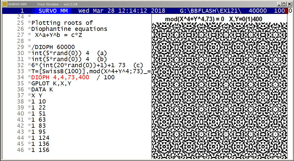
This demo in YouTube
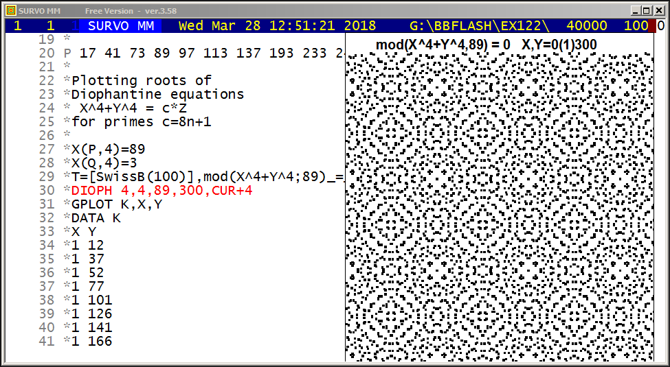
This demo in YouTube
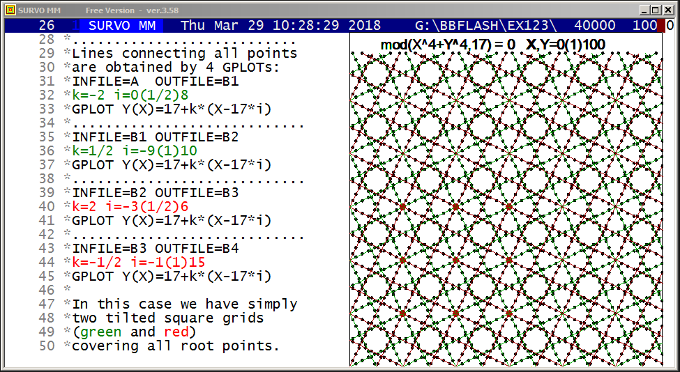
This demo in YouTube
The connections between the roots of the Diophantine equation
X^4+Y^4=17*Z are studied and it will be seen that they are located
in the integer points of lines of type
Y=17+k*(X-17*i), k=-2, -1/2, 1/2, 2
and thus forming two slanted grids of squares.
Obviously similar results are obtained in cases X^4+Y^4=c*Z
when c is a prime of the form c=h*(8*n+1).
This is trivially true for other values of c.
Mathematical background information
More examples of cases X^4+Y^4=c*Z where c=8n+1 is as prime or a product of such primes
For c=8*11+1=89 the grid lines have slopes k=-7/5, 5/7, -5/7, 7/5.

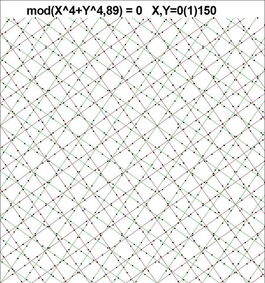
For c=8*9+1=73 the grid lines have slopes k=-7/3, 3/7, 7/3, -3/7.
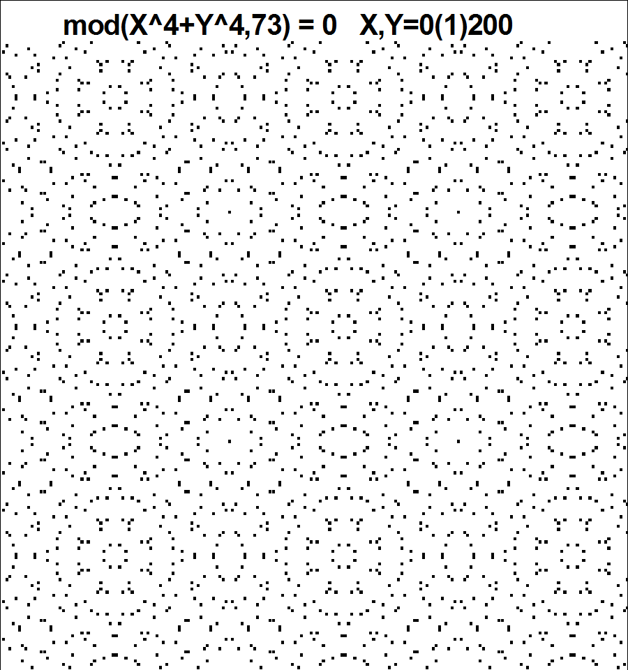
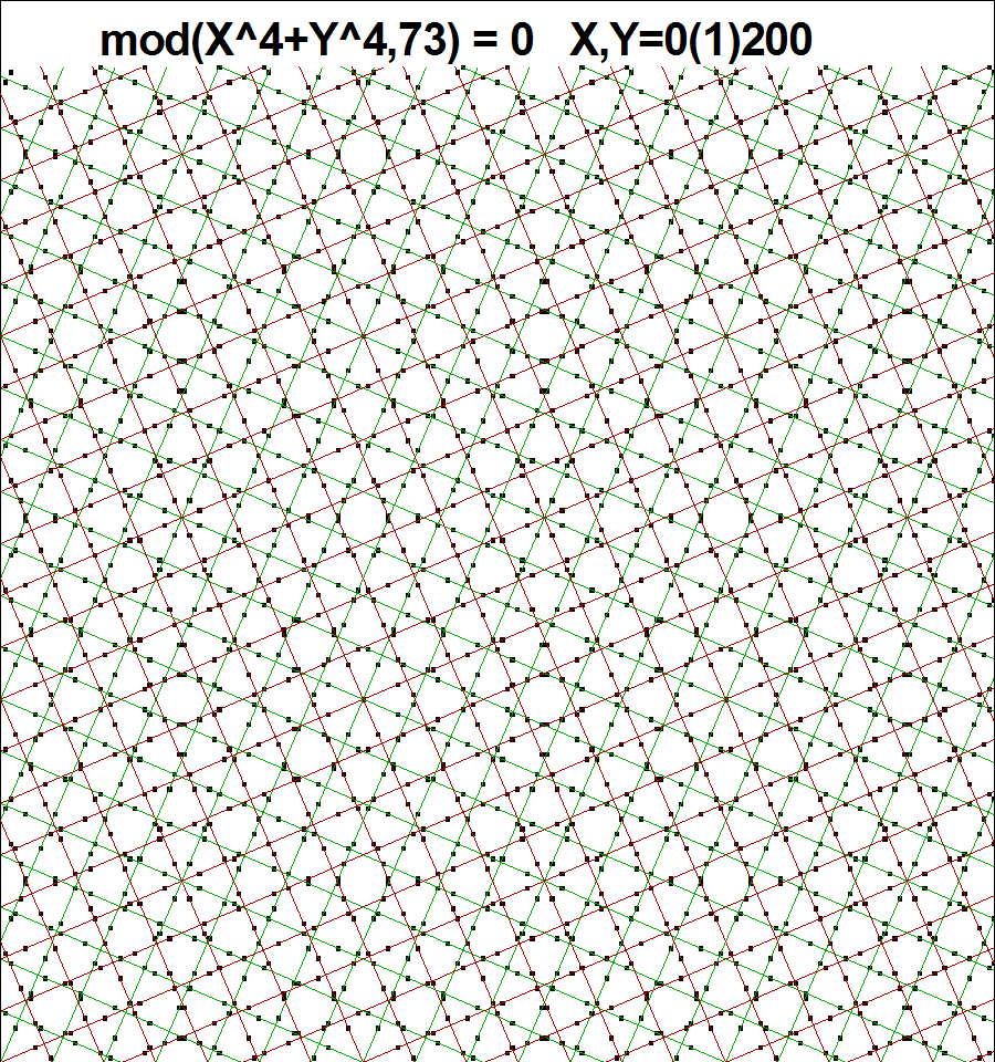
For c=8*54+1=433 the grid lines have slopes k=-1/3, 3, 1/3, -3.
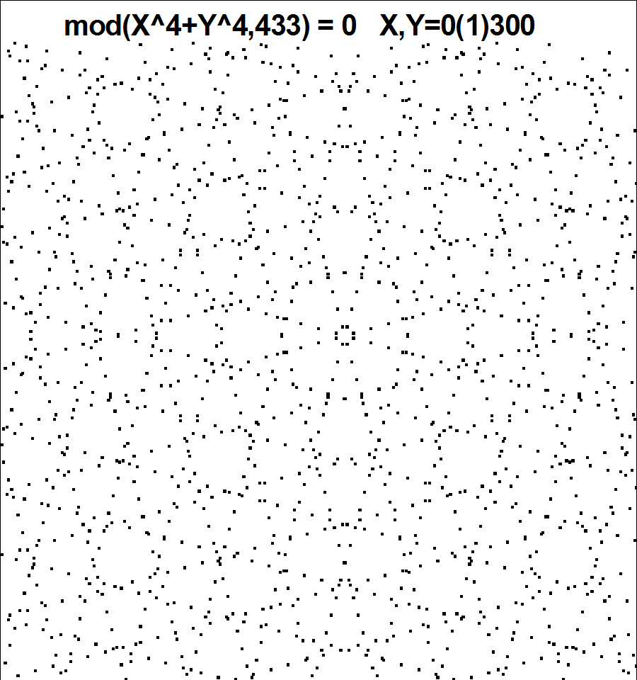
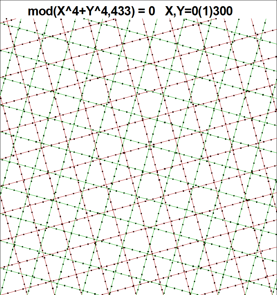
Graph of case c=697=17*41:
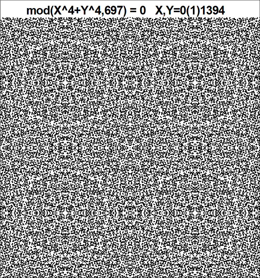
Combination of mod(X^4+Y^4,c)=0 and mod(X^2+Y^4,c)=0 for c=1049:
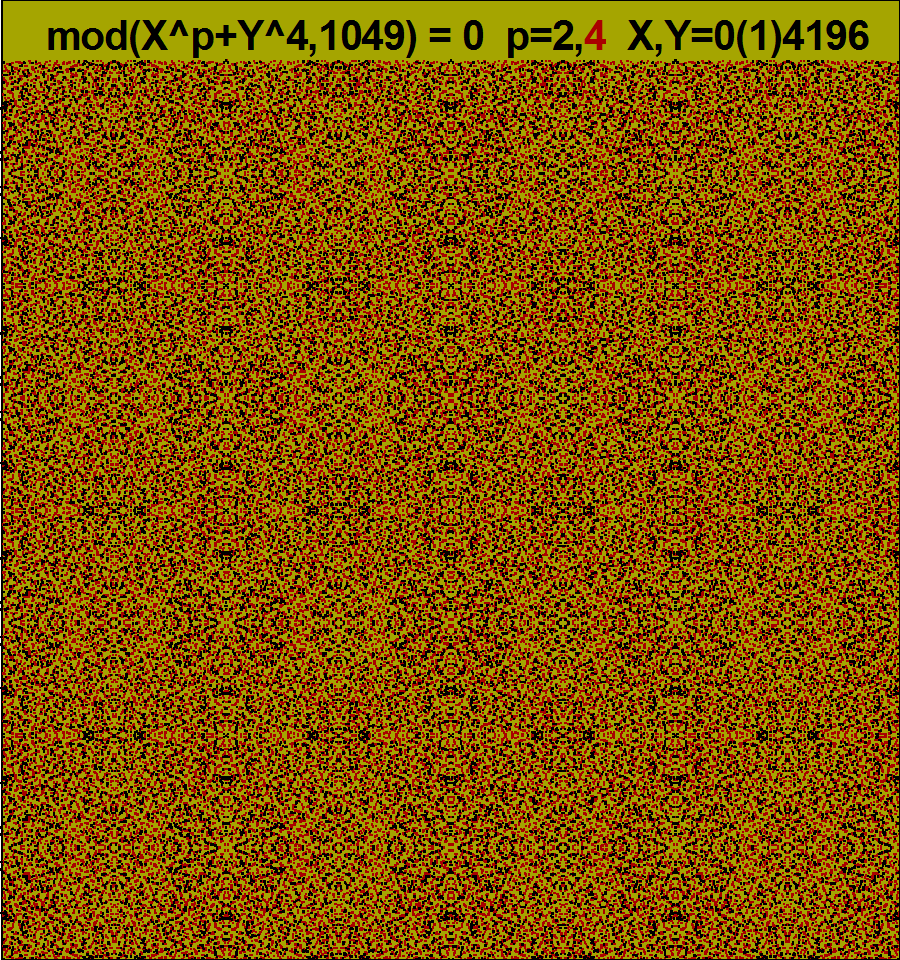
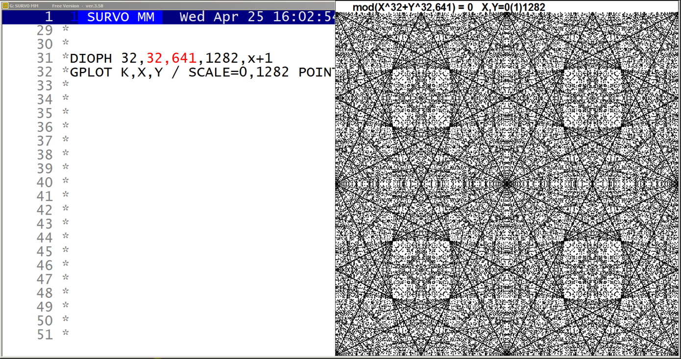
This demo in YouTube
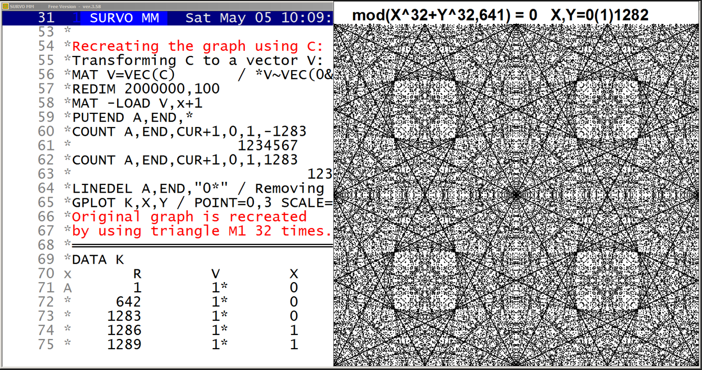
This demo in YouTube
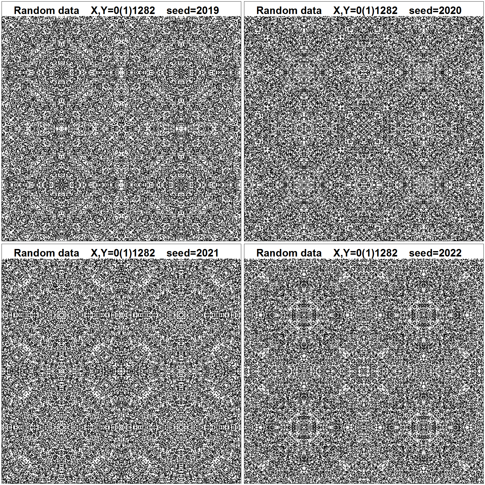
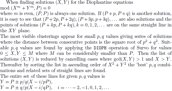
*TUTSAVE DIOPH
/
/ def Wm=W1 Wm2=W2 Wprime=W3 Wn=W4
/
*{R}
*SCRATCH {act}{home}
*DIOPH {write Wm},{write Wm2},{write Wprime},{write Wn},CUR+4{act}
*{R}
*FILE COPY DIOPH1 TO NEW DIOPH{R}
*DATA DIOPH1{R}
*p q{R}
/  The results of DIOPH are saved{R}
/  in a Survo data file DIOPH as variables p,q.{R}
*{u3}{act}
*SCRATCH {act}{home}
*VAR G:2=gcd(p,q) TO DIOPH{act}{R}
*VAR C1:1=if(p>q)then(0)else(1) TO DIOPH{act}{R}
*VAR C2:1=if(G>1)then(0)else(1) TO DIOPH{act}{R}
*VAR C3:1=C1*C2 TO DIOPH{act}{R}
*FILE COPY DIOPH TO NEW DIOPH2 / IND=C3,1{act}{R}
*VAR R:2=sqrt(p*p+q*q) TO DIOPH2{act}{R}
*FILE SORT DIOPH2 BY R TO DIOPH3{act}{R}
*FILE LOAD DIOPH3 / IND=ORDER,2,20 VARS=p,q,R{act}
*{end}
/DIOPH 32,32,641,100
DIOPH 32,32,641,100,CUR+4                         / n_comb=533
  The results of DIOPH are saved
  in a Survo data file DIOPH as variables p,q.
VAR G:2=gcd(p,q) TO DIOPH
VAR C1:1=if(p>q)then(0)else(1) TO DIOPH
VAR C2:1=if(G>1)then(0)else(1) TO DIOPH
VAR C3:1=C1*C2 TO DIOPH
FILE COPY DIOPH TO NEW DIOPH2 / IND=C3,1
VAR R:2=sqrt(p*p+q*q) TO DIOPH2
FILE SORT DIOPH2 BY R TO DIOPH3
FILE LOAD DIOPH3 / IND=ORDER,2,20 VARS=p,q,R
DATA DIOPH3*,A,B,C
   p   q      R
   1   2      2
   1   5      5
   4   5      6
   1   8      8
   9  13     15
   5  16     16
   1  20     20
   2  25     25
   8  25     26
  17  27     31
   1  32     32
  21  31     37
  13  36     38
  19  33     38
  23  33     40
  25  32     40
   3  41     41
  12  41     42
  29  31     42
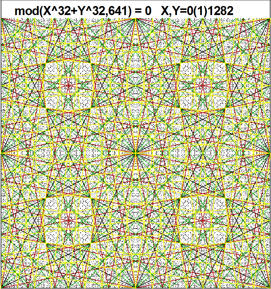
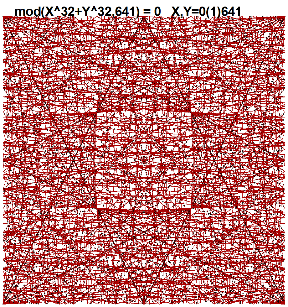
  m    2^m   P   ratios
  2    4    17   1/2
  3    8    97   1/8   5/7
  4   16   929   11/12 4/17 7/25 14/29
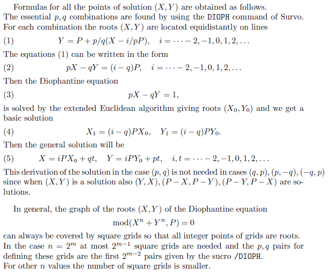
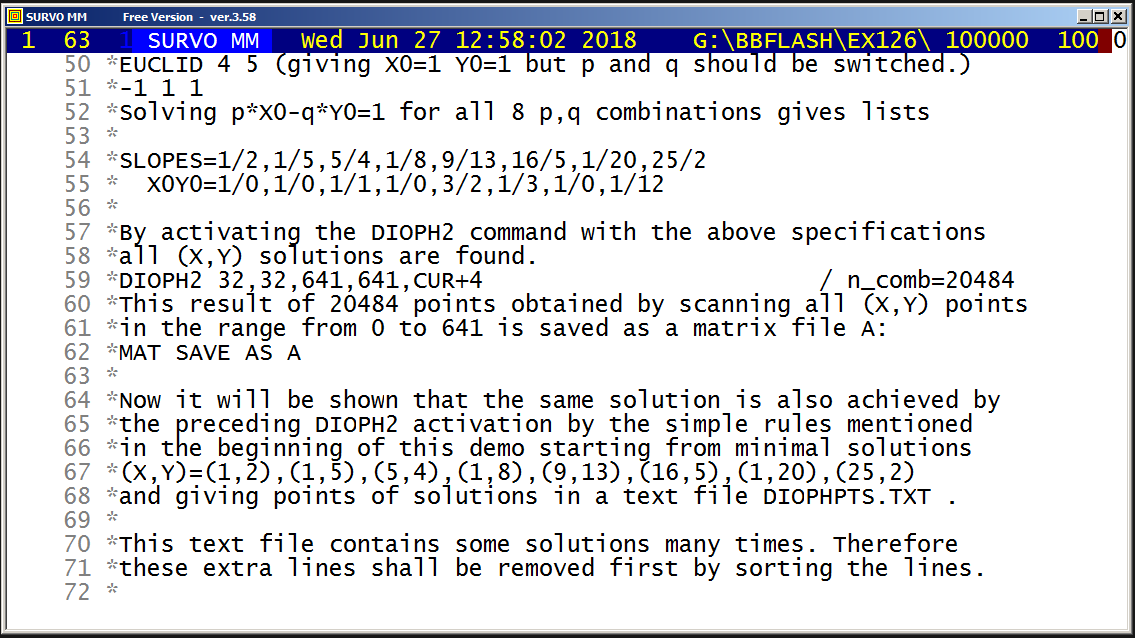
This demo in YouTube
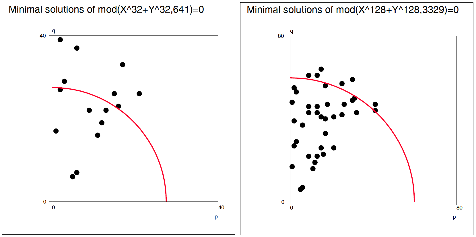
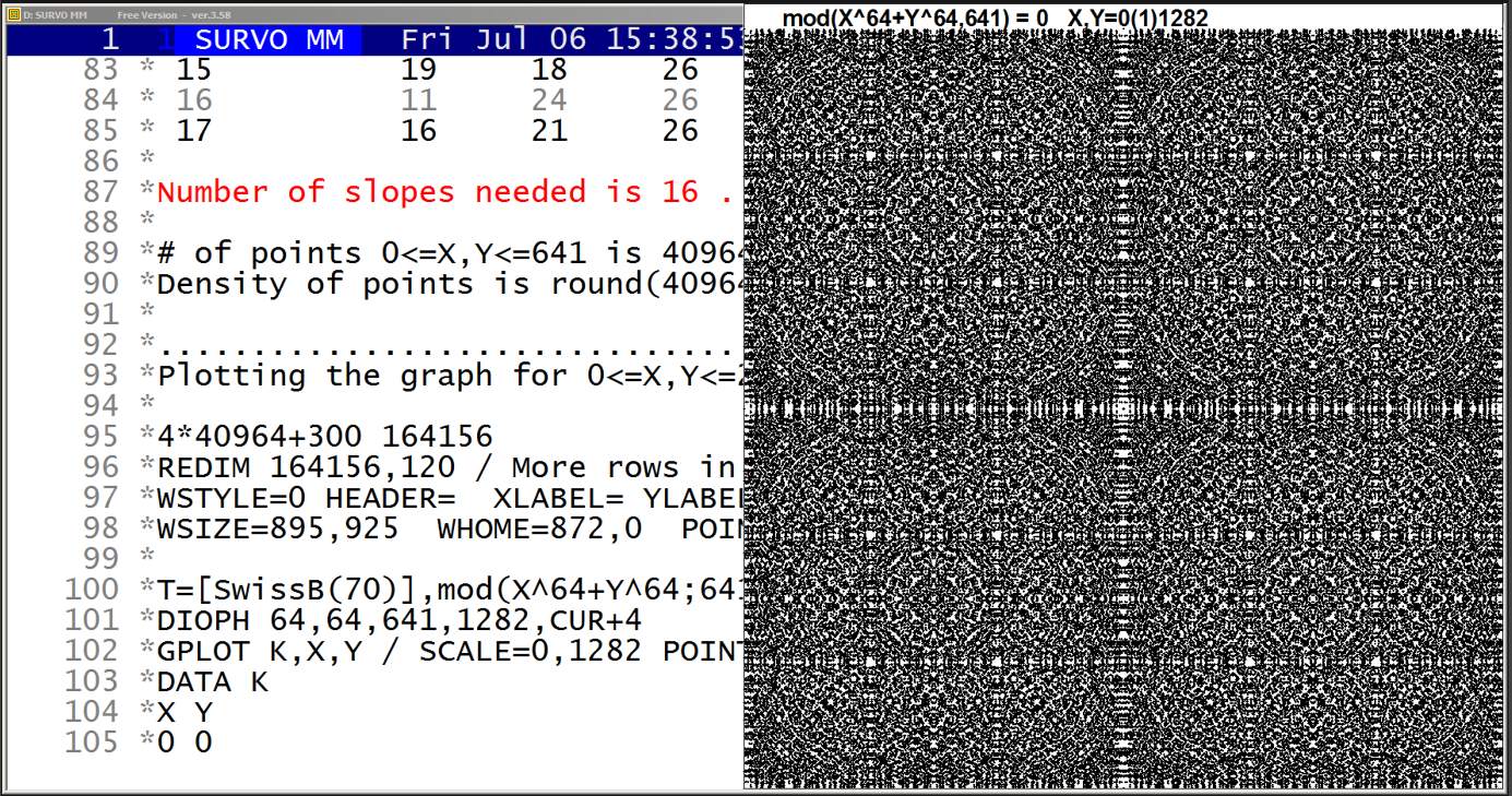
This demo in YouTube
For n=32, P=641 we have

criterion          p,q ratios

sqrt(p^2+q^2)      1/2 1/5 4/5 1/8  9/13 5/16 1/20 2/25
(p^4+q^4)^(1/4)    1/2 1/5 1/8 1/20 4/5  1/50 2/25 5/16
min(p,q)           1/2 1/5 1/8 1/20 1/50 1/77 1/125 1/129

Table of p,q values for min(p,q):

///           p      q      R     X0     Y0  valid
  1           1      2      1      1      0      1
  2           1      5      1      1      0      1
  3           1      8      1      1      0      1
  4           1     20      1      1      0      1
  5           1     32      1      1      0      0
  6           1     50      1      1      0      1
  7           1     77      1      1      0      1
  8           1     80      1      1      0      0
  9           1    125      1      1      0      1
 10           1    128      1      1      0      0
 11           1    129      1      1      0      1

so that 3 suggested combinations are unnecessary.
n=5, P=701, gcd(n,P-1)=5
(p,q) = (-1,1) (1,4) (2,5)
               (4,1) (5,2)

n=9, P=73 , gcd(n,P-1)=9
(p,q) = (-1,1) (-1,2) (-1,4) (8,9) (4,9)
               (-2,1) (-4,1) (9,8) (9,4)

n=15, P=701, gcd(n,P-1)=5
(p,q) = (-1,1) (-8,11) (3,10)
               (-11,8) (10,3)

n=11, P=199, gcd(11,199-1)=11
(p,q) = (-1,1) (3,10) (1,11) (3,13) (11,18) (-2,7)
               (10,3) (11,1) (13,3) (18,11) (-7,2)

n=13, P=157, gcd(n,P-1)=13
(p,q) = (-1,1) (1,4) (2,7) (5,6) (3,11) (10,11) (9,13)
               (4,1) (7,2) (6,5) (11,3) (11,10) (13,9)

n=17, P=239, gcd(n,P-1)=17
(p,q) = (-1,1) (7,9) (7,10) (3,14) (9,13) (10,13) (11,14) (10,19) (-1,6)
               (9,7) (10,7) (14,3) (13,9) (13,10) (14,11) (19,10) (-6,1)
  i   p   q  mod(p^n,P) mod(q^n,P)   sum

  1   3  11  169        472          641
  2   6  11  169        472          641
  3  12  11  169        472          641
  4  15  11  169        472          641
  5   1  21    1        640          641
  6  19   9  284        357          641
  7  21   2  640          1          641
  8  21   4  640          1          641
  9  21   5  640          1          641
 10  22   3  472        169          641
 11   8  21    1        640          641
 12  13  19  357        284          641
 13  21  10  640          1          641
 14  23   9  284        357          641
 15  19  18  284        357          641
 16  11  24  472        169          641
 17  16  21    1        640          641
Then instead of scanning a lot of X,Y combinations it is sufficient to tabulate values mod(X^n,P), X=1,2,... and to find out X,Y combinations satisfying mod(X^n,P)+mod(Y^n,P)=P.
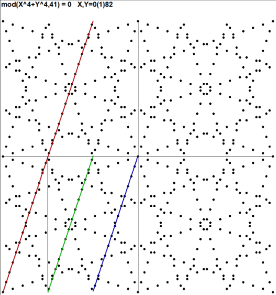
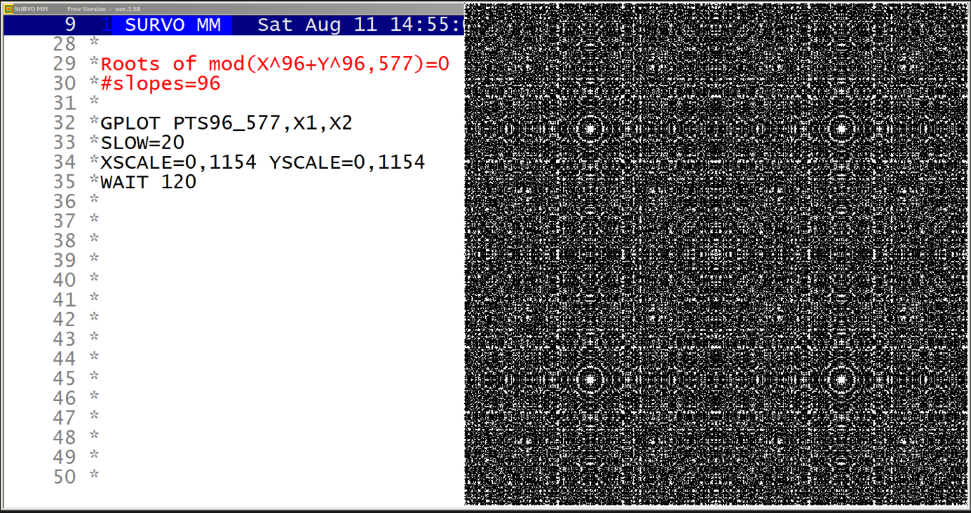
This demo in YouTube
For example, the last scatter diagram related to mod(X^96+Y^96,577)=0
was created in the following way:

POINTS2=1 / Save points (X,Y) of solution as a text file POINTS2.TXT
/D_SOLVE0 96,96,577,100,30

When the above sucro command was activated, it gave following output:
(corrected 31 March 2022)
..................................................
Solving Diophantine equation mod(X^96+Y^96,577)=0

Matrix PQ_X0Y0 of p,q,X0,Y0 values created!
Computing roots:
SLOPES=PQ_X0Y0 POINTS=A96_577.TXT
DIOPH3 96,96,577,577,CUR+1

Number of slopes needed is 24 .

Values of p,q,R,X0,Y0 for these 24 slopes are:

///           p      q      R     X0     Y0
  1           5      2      5      1      2
  2           6      5      8      1      1
  3           4      7      8      2      1
  4          13      4     14      1      3
  5          12      7     14      3      5
  6           1     14     14      1      0
  7           3     14     14      5      1
  8          15      2     15      1      7
  9          14      9     17      2      3
 10          16      5     17      1      3
 11          13     12     18      1      1
 12           5     17     18      7      2
 13          14     11     18      4      5
 14          18      5     19      2      7
 15           1     20     20      1      0
 16           3     20     20      7      1
 17          21      4     21      1      5
 18           9     20     22      9      4
 19          16     15     22      1      1
 20           5     22     23      9      2
 21          15     17     23      8      7
 22          20     11     23      5      9
 23          19     14     24      3      4
 24           7     23     24     10      3

..................................................

In the above run the command
DIOPH3 96,96,577,577,CUR+1
created also the sequence of solutions (X,Y) in the order
they were found and saved them in the text file POINTS2.TXT.
When in this process a solution (X,Y) was found, also its companion
solutions (Y,X),(X,P-Y),(P-Y,X),(P-X,Y),(Y,P-X),(P-X,P-Y),(P-Y,P-X)
for P=577 were saved in POINTS2.TXT.
Then the final graph emerges as a series of symmetric subgraphs.

Thereafter the graphical output was generated in this way:

FILE SAVE POINTS2.TXT TO PTS96_577 / Conversion to a data file

GPLOT PTS96_577,X1,X2
SLOW=20 / slowing down the plotting process
XSCALE=0,1154 YSCALE=0,1154

WHOME=846,2 WSIZE=920,920 HEADER=  MODE=2000,2000
POINT=0,3 WSTYLE=0 XDIV=0,1,0 YDIV=0,1,0 FRAME=0 XLABEL= YLABEL=
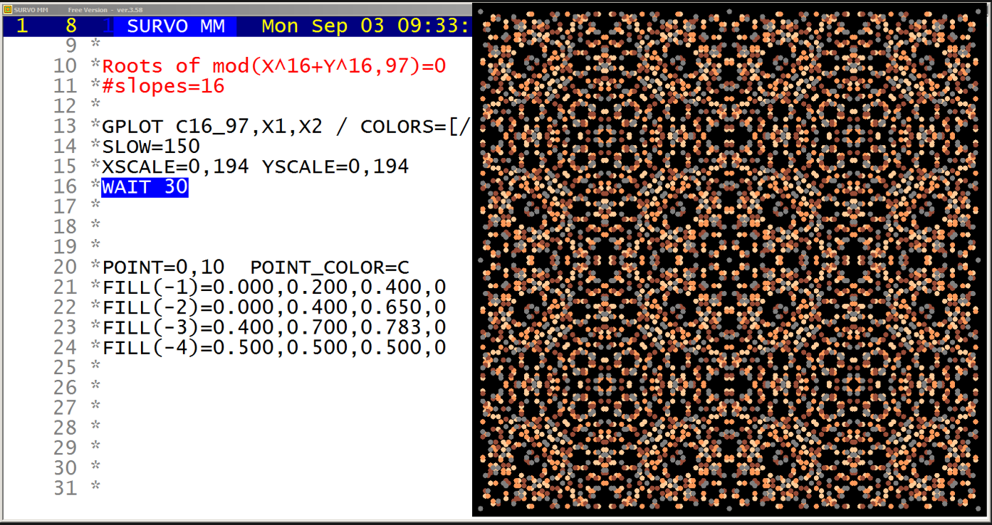
This demo in YouTube
Another set of 12 colored textures by roots
of Diophantine equations mod(X^n+Y^n,P)=0
in YouTube
POINTS2=1 COLOR=1
/D_SOLVE0 16,16,97,100,30

Solving Diophantine equation mod(X^16+Y^16,97)=0

SLOPES=PQ_X0Y0 POINTS=A16_97.TXT
DIOPH3 16,16,97,97,CUR+1

Number of slopes needed is 4 .

Values of p,q,R,X0,Y0,valid for these 4 slopes are:
///           p      q      R     X0     Y0  valid
  1           5      2      7      1      2      1
  2           3      5      8      2      1      1
  3           7      2      9      1      3      1
  4           7      3     10      1      2      1
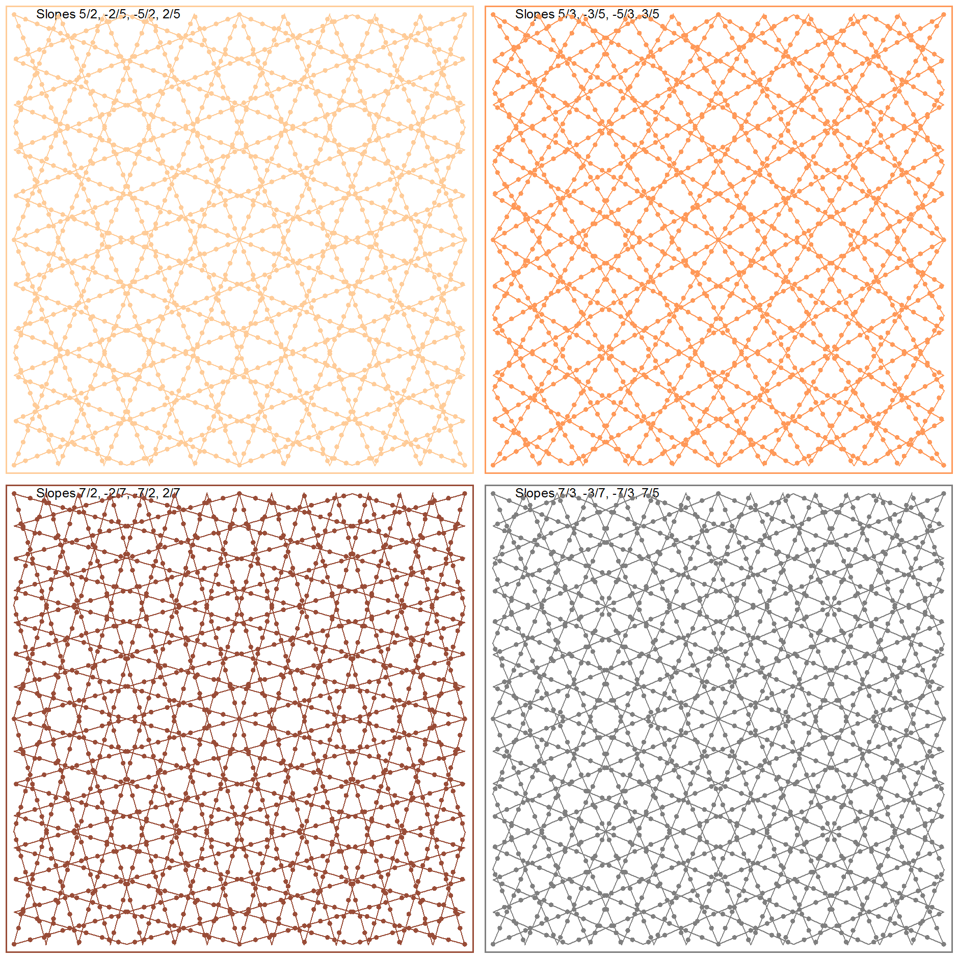
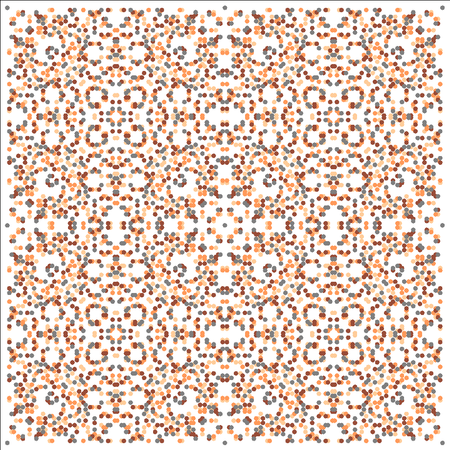
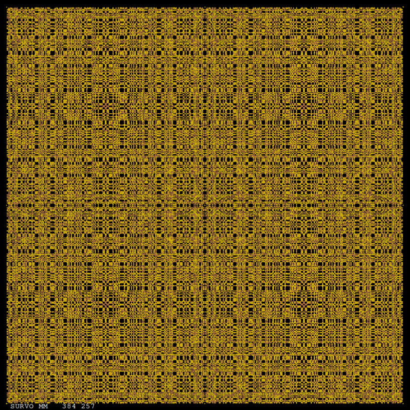
This demo in YouTube
The graphs of the roots of Diophantine equations mod(X^n+Y^n,P)=0 for
twelve pairs of n and P values are are displayed stepwise in multiple
colors. The roots related to the same p,q values (described in previous
demos) have the same color.
In this way the structure of these graphs
related to several overlayed slanted square grids becomes more obvious.
More information about this topic is given in the comments of the
previous demo
Colored textures by roots of mod(X^n+Y^n,P)=0
Seppo Mustonen: On the roots of nonlinear Diophantic equations mod(X^n+Y^n,P)=0 (2018)
Mathematical background information
Still another set of
12 examples in YouTube
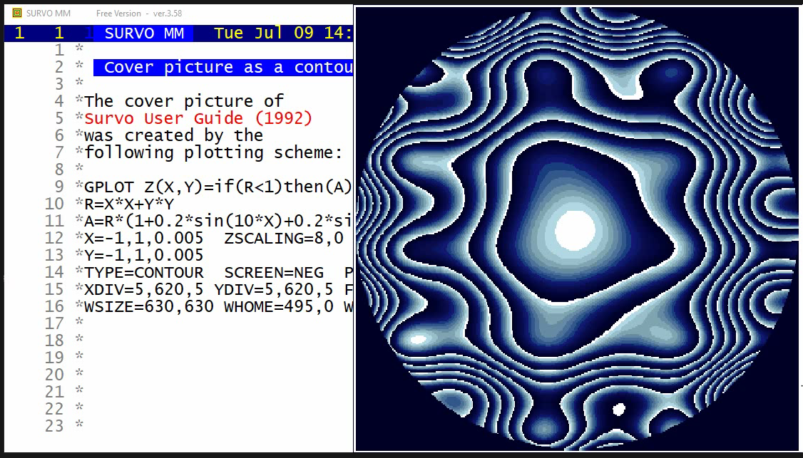
This demo in YouTube
The cover picture of the
Survo User Guide
(1992) is presented in various forms.
Animation of the cover picture of Survo User's guide
(Start the demo by clicking the picture below!)
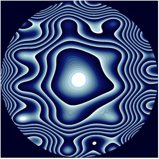
This animation in YouTube
The function plotted in this demo is
f(x,y)=(x^2+y^2)*(1+a*sin(10*x)+a*sin(b*y)
for a=0(0.002)0.2 and b=10(0.05)15 simultaneously.
Then the final graph (a=0.2, b=15) is the cover picture.
The 101 frames of this movie were created by the following setup
in an edit field of Survo
*
*R=X*X+Y*Y
*X=-1,1,0.005  ZSCALING=8,0
*Y=-1,1,0.005
*TYPE=CONTOUR  SCREEN=NEG  PALETTE=VGABLUE
*XDIV=0,1000,0 YDIV=0,1000,0 FRAME=3 HEADER=
*WSIZE=1000,1000 WHOME=1000,0 WSTYLE=0
*
*TUTSAVE MOVIE
/
*{W1=0}{W2=10}{W3=0}{W4=100000}{tempo -1}{R}
+ A:
*{erase}A=R*(1+{write W1}*sin(10*X)+{write W1}*sin({write W2}*Y)){R}
*{erase}OUTFILE=P{W3=W3+1}{W4=W3+100000}{write W4}{l6}{del}{R}
*{erase}GPLOT Z(X,Y)=if(R<1)then(A)else(2047/2048){act}
*{tempo +1}{10000}{tempo -1}
*{W1=W1+0.002}{W2=W2+0.05}{R}
*GPLOT /DEL ALL{act}{home}{u3}{goto A}
*{end}
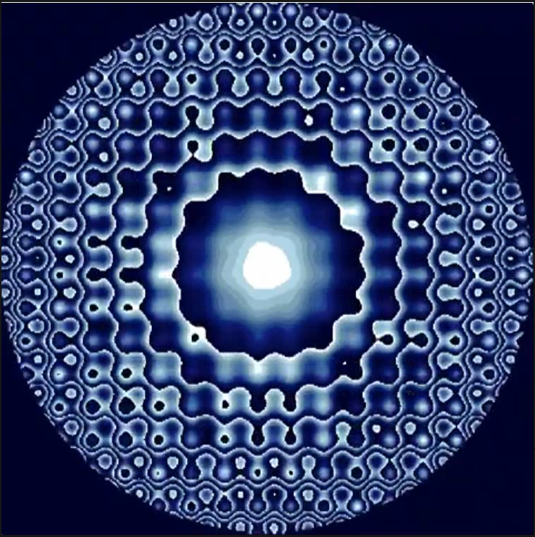
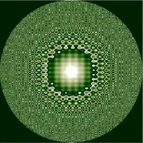
*Frames of the first half of this extension were created by the sucro MOVIE:
*
*TUTSAVE MOVIE
*{W1=0}{W2=0}{R}
+ A: {W2=W2+1}
*{erase}A=R*(1+0.2*sin({write W1}*X)+0.2*sin(1.5*{write W1}*Y)){R}
*{erase}OUTFILE=P{write W2}{R}
*{erase}GPLOT Z(X,Y)=if(R<1)then(A)else(2047/2048){act}
*{100}{R}
*>magick convert -scale x%182 P{write W2}.emf P{write W2}.png{act}{R}{30}
*>DEL P{write W2}.emf{act}{10}{R}
*{W1=W1+0.1}
*GPLOT /DEL ALL{act}{home}{u5}{goto A}
*{end}
*
*The second half was made from the first half by copying frames in
*opposite order.
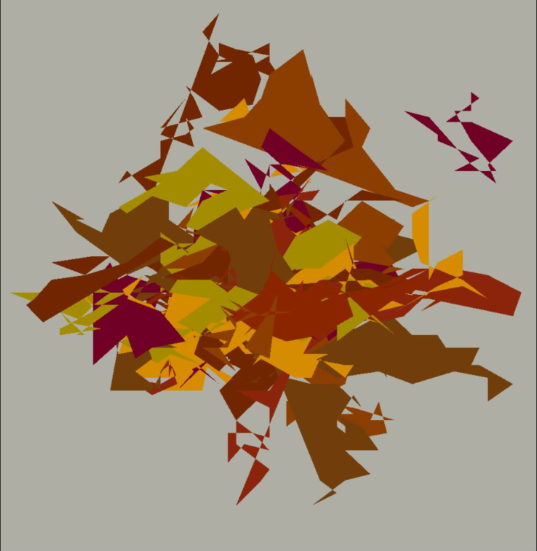
This demo in YouTube
This is the cover picture of Guide for SURVO MM installation and setup (2002 in Finnish)
in a slightly animated form.
The graph is created by the following setup of Survo:
  1 *
  2 */ACTIVATE +
  3 +FILE MAKE POLY,4,2000,X,2
  4 *A=10
  5 +VAR X1,X2,X3,X4 TO POLY
  6 *X1=if(ORDER=1)then(0)else(X1[-1]+A*(0.5-rand(2002)))
  7 *X2=if(ORDER=1)then(0)else(X2[-1]+A*(0.5-rand(2002)))
  8 *X3=-1-8*rand(2002)
  9 *X4=if(ORDER=1)then(1)else(X41)
 10 *X41=if(X4[-1]<10)then(X4[-1]+2*rand(2002))else(0)
 11 *...........
 12 +VAR X1,X2 TO POLY
 13 *X1=if(X4>0)then(X1)else(X3)
 14 *X2=if(X4>0)then(X2)else(MISSING)
 15 *...........
 16 +GPLOT POLY,X1,X2
 17 *LINE=POLYGON,5   FRAME=0 XDIV=0,1,0 YDIV=0,1,0 HEADER= XLABEL= YLABEL=
 18 *WHOME=5,0  WSIZE=965,992 WSTYLE=0  XSCALE=-32,32 YSCALE=-43,48
 19 *FRAMES=F F=0,0,639,350,-9          LINETYPE=[line_width(0)][WHITE]
 20 *FILL(-1)=0.0,0.3,1.0,0.15
 21 *FILL(-2)=0.1,0.5,0.6,0.35
 22 *FILL(-3)=0.2,0.4,0.6,0.35
 23 *FILL(-4)=0.1,0.5,0.9,0.35
 24 *FILL(-5)=0.0,0.1,0.7,0.35
 25 *FILL(-6)=0.2,0.7,0.5,0.35
 26 *FILL(-7)=0.1,0.4,0.8,0.35
 27 *FILL(-8)=0.2,0.5,0.9,0.35
 28 *
 29 *FILL(-9)=0.01,0.01,0.05,0.30 / background
 30 *
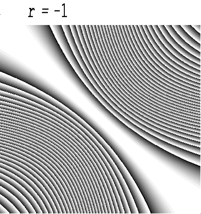
This demo in YouTube for -1 ≤ r ≤ 2
Influence curves of the correlation coefficient r are shown
for increasing values of r when the sample size is 30,
means of variables are 0 and standard deviations are 1
for -10 ≤ X,Y ≤ 10.
Formulas and background information are given in an earlier demo
Influence curves for the correlation coefficient
It is interesting to see these graphs also when r exceeds 1,
but then they are statistically meaningless.
Here are some examples with very large r values:
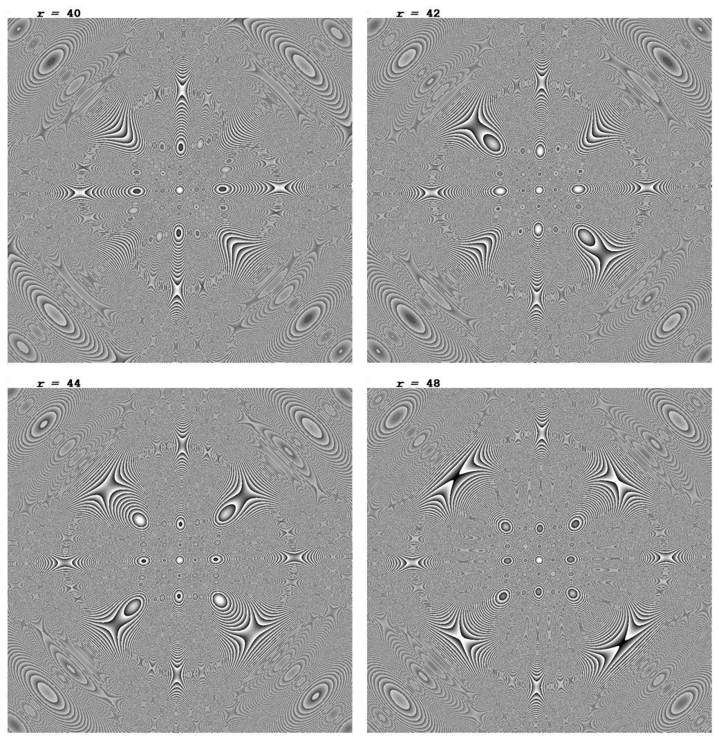
The graphs were created by the following setup in the edit field of Survo:
 10 *   *GLOBAL*
 11 *WSIZE=1000,1020 WHOME=893,0   videomode=1000,1020
 12 *XSCALE=-10,0,10 YSCALE=-10,0,10 XDIV=0,1000,0 YDIV=0,1000,20
 13 *WSTYLE=0 FRAME=0 HEADER=
 14 *X=-10,10,0.02 Y=-10,10,0.02
 15 *
 16 *mx=0 my=0 sx=1 sy=1 n=30
 17 *  z(x,y)=abs(r*(1-w)+u*v)/w
 18 *  u=sqrt(n/(n*n-1))*(X-mx)/sx
 19 *  v=sqrt(n/(n*n-1))*(Y-my)/sy
 20 *  w=sqrt((1+u*u)*(1+v*v))
 21 *
 22 *TYPE=CONTOUR SCREEN=NEG ZSCALING=20,0
 23 *PALETTE=VGAGRAY.PAL
 24 *TEXTS=T1,T2
 25 *T1=[CourierBI(40)],___r_=_,20,993
 26 *
 27 *TUTSAVE MOVIE
 28 /
 29 *{W1=0}{W2=0}{R}
 30 + A: {tempo -1}{erase}SYSTEM videomode=1000,1020{act}{R}
 31 *{W2=W2+1}
 32 *{erase}OUTFILE=P{write W2}{R}
 33 *T2=[CourierB(40)],{write W1},170,993{R}
 34 *{erase}GPLOT z(X,Y)=abs({write W1}*(1-w)+u*v)/w{tempo +1}{act}
 35 *{wait 350}{R}
 36 *{erase}>magick convert P{write W2}.emf P{write W2}.png
 37 *{act}{R}
 38 *{wait 30}{erase}>DEL P{write W2}.emf{act}{wait 10}{R}
 39 *{W1=W1+1}GPLOT /DEL ALL{act}{home}{u6}{goto A}
 40 *{end}
 41 *
 42 *................................................
 43 *
 44 */MOVIE
 45 *SYSTEM videomode=1000,1020
 46 *OUTFILE=P1
 47 *T2=[CourierB(40)],0,170,993
 48 *GPLOT z(X,Y)=abs(0*(1-w)+u*v)/w
 49 *>magick convert P1.emf P1.png
 50 *>DEL P1.emf
 52 *GPLOT /DEL ALL
 52 *
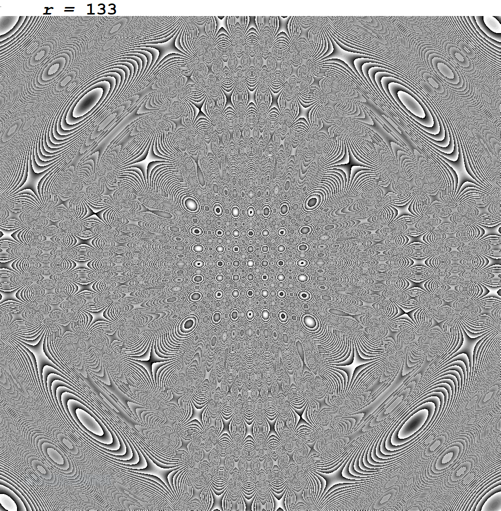

This demo in YouTube
It is shown how Survo Puzzles are solved by a
Javascript application.
Thirty examples with solutions
Try to solve them without looking to solutions.
You may also create new
problems just by giving codes of the form xyz-aaaaa where
x=# of rows, y=# of columns, z=max.number of swaps needed, and
aaaaa=serial number.
Try to solve the following Survo Puzzles by
Javascript application.
353-858
443-123
363-560
343-878
Other demos about Survo puzzles:
Solving a Survo puzzle
Solving a Survo puzzle by swapping
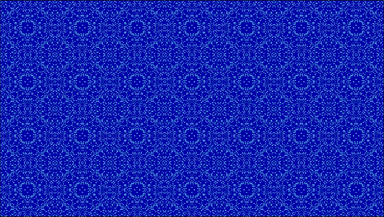
This demo in YouTube
In earlier demos the roots of equations mod(X^n+Y^n,P)=0
have been plotted for non-negative X,Y values less than 2P.
Here the area has been extended to X values less than 7P
and Y values less than 4P.
Seppo Mustonen: On the roots of nonlinear Diophantic equations mod(X^n+Y^n,P)=0 (2018)
Seppo Mustonen: Diophantine equations mod(X^n+Y^n,P)=0, additional results and graphical presentations (2022)
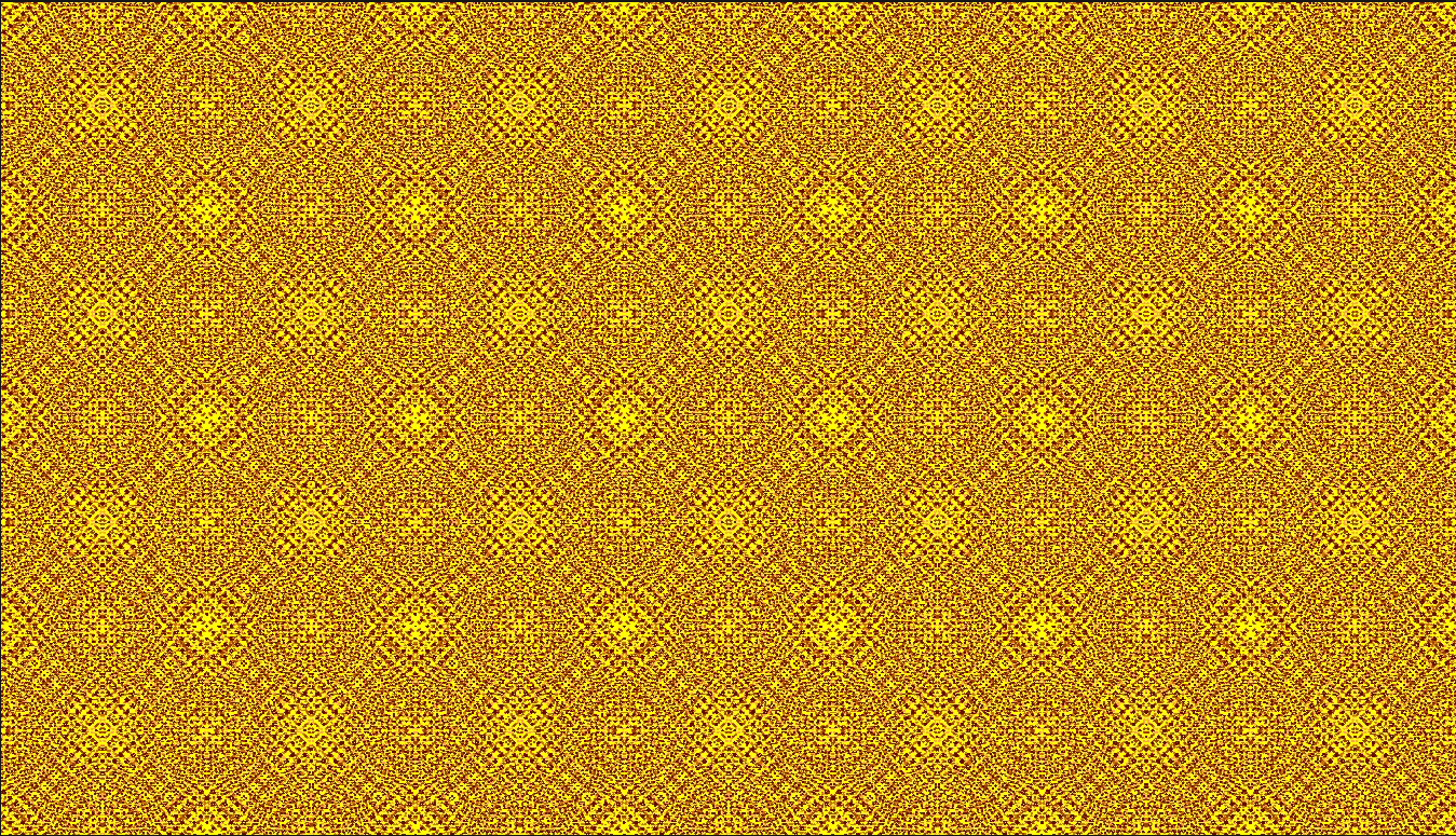
This demo in YouTube
In earlier demos the roots of equations mod(X^n+Y^n,P)=0
have been plotted for non-negative X,Y values less than 2P.
Here the area has been extended to X values less than 7P
and Y values less than 4P.
In the 11th example mod(X^2+Y^2,85)=0 the parameter P=85=5*17 is not
a prime. In this case the standard slopes are 7/6,-6/7,9/2,-2/9, but
also slopes -7/6,6/7,-9/2,2/9 are needed for covering all roots.
In the graph below the covering lines are plotted for 0<=X,Y<=P .
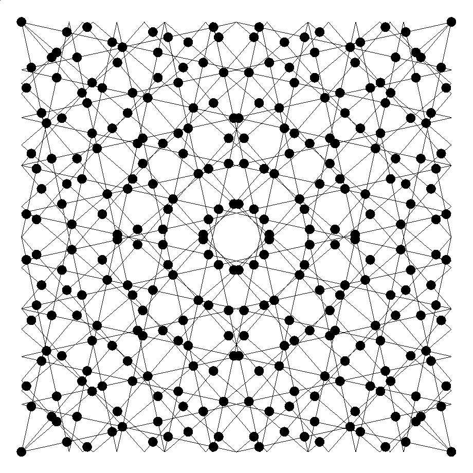
4 Aug 2022
In fact each inner point in the graph is covered by two lines
orthogonally. Therefore all points are covered by ascending lines
with slopes 7/6, 6/7, 9/2, 2/9
Seppo Mustonen: On the roots of nonlinear Diophantic equations mod(X^n+Y^n,P)=0 (2018)
Seppo Mustonen: Diophantine equations mod(X^n+Y^n,P)=0, additional results and graphical presentations (2022)
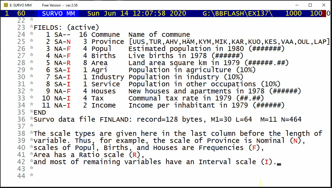
This demo in YouTube
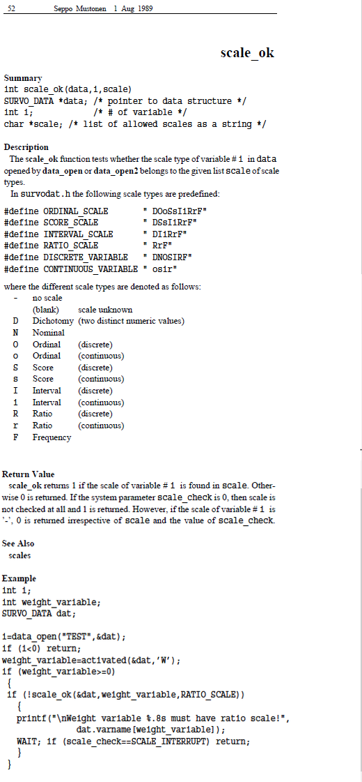
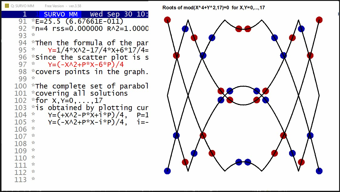
This demo in YouTube
After finding interesting structural properties for the roots
of Diophantine equations X^n+Y^n ≡ 0 (mod P) by making computational
experiments by using Survo, I tried to study equations
X^4+Y^2 ≡ 0 (mod P) in a similar way.
Since in the previous case the structures of solutions were linear,
it was natural to expect quadratic structures in this new case.
When trying to use higher degree polynomials as models
in the general
ESTIMATE operation
of Survo, the coefficients
in terms above degree 2 turned out to be zeros.
Diophantine equations of the form X^4+Y^2 ≡ 0 (mod P) have nontrivial
solutions for primes P of the form P=4k+1.
By making numerical experiments by means of Survo it is found that
the roots 0<=X,Y<=P for a given P are integer points on parabolas
Y=[+-(X^2-P*X)+P*i]/C(P)
where i is any integer and
C(P) is the minimal integer square root of -1 modulo P
documented as sequence A002314 in OEIS.
I have tested this result for the 16 first primes of the form P=4k+1
and below is a list of them with corresponding C(P) values.
 P     5,13,17,29,37,41,53,61,73,89,97,101,109,113,137,149
 C(P)  2, 5, 4,12, 6, 9,23,11,27,34,22, 10, 33, 15, 37, 44
DATA XYIL
 X  Y    I  L
 0  0    2  0    I1(0,0)=0
 0 17    1  4    I1(0,17)=4
 1  4    2  0    I1(1,4)=1.8823529411765   I2(1,4)=0
 1 13    1  4    I1(1,13)=4
 2  1    1  2    I1(2,1)=2
 2 16    2  2    I1(2,16)=5.5294117647059  I2(2,16)=2
 3  2    2 -2    I1(3,2)=2.9411764705882   I2(3,2)=-2
 3 15    1  6    I1(3,15)=6
 4  4    1  4    I1(4,4)=4
 4 13    2  0    I1(4,13)=6.1176470588235  I2(4,13)=0
 5  2    1  4    I1(5,2)=4
 5 15    2  0    I1(5,15)=7.0588235294118  I2(5,15)=0
 6  8    2 -2    I1(6,8)=5.7647058823529   I2(6,8)=-2
 6  9    1  6    I1(6,9)=6
 7  8    1  6    I1(7,8)=6
 7  9    2 -2    I1(7,9)=6.2352941176471   I2(7,9)=-2
 8  1    2 -4    I1(8,1)=4.4705882352941   I2(8,1)=-4
 8 16    1  8    I1(8,16)=8
 9  1    2 -4    I1(9,1)=4.4705882352941   I2(9,1)=-4
 9 16    1  8    I1(9,16)=8
10  8    1  6    I1(10,8)=6
10  9    2 -2    I1(10,9)=6.2352941176471  I2(10,9)=-2
11  8    2 -2    I1(11,8)=5.7647058823529  I2(11,8)=-2
11  9    1  6    I1(11,9)=6
12  2    1  4    I1(12,2)=4
12 15    2  0    I1(12,15)=7.0588235294118 I2(12,15)=0
13  4    1  4    I1(13,4)=4
13 13    2  0    I1(13,13)=6.1176470588235 I2(13,13)=0
14  2    2 -2    I1(14,2)=2.9411764705882  I2(14,2)=-2
14 15    1  6    I1(14,15)=6
15  1    1  2    I1(15,1)=2
15 16    2  2    I1(15,16)=5.5294117647059 I2(15,16)=2
16  4    2  0    I1(16,4)=1.8823529411765  I2(16,4)=0
16 13    1  4    I1(16,13)=4
17  0    2  0    I1(17,0)=0
17 17    1  4    I1(17,17)=0               I2(17,17)=4
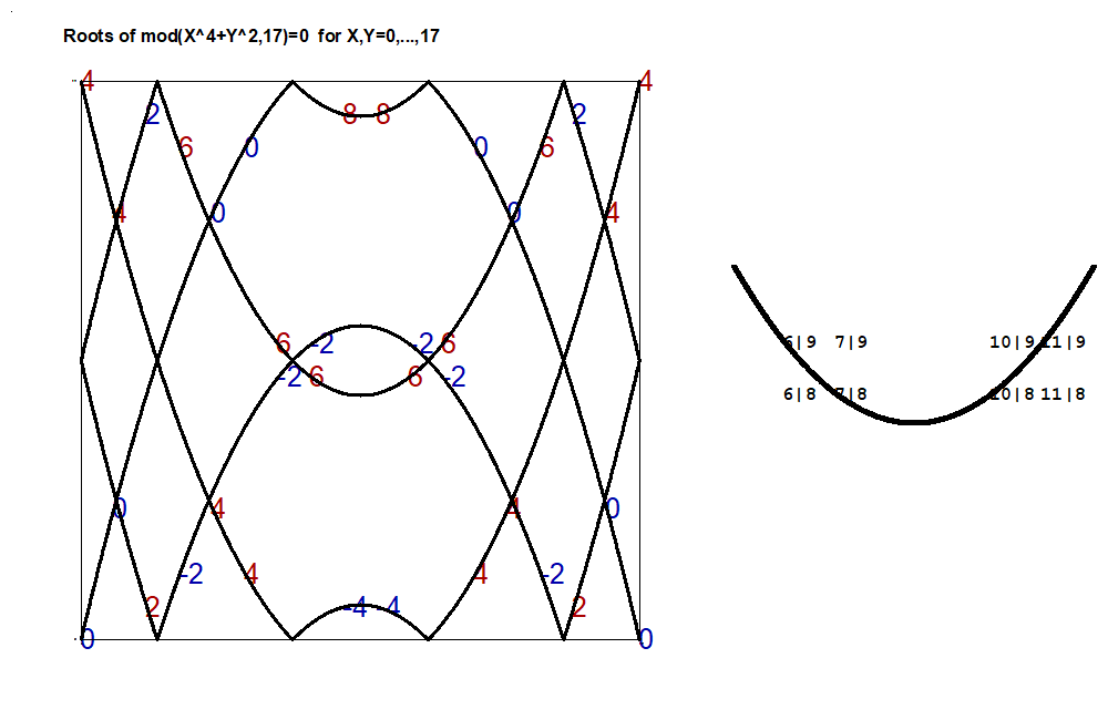
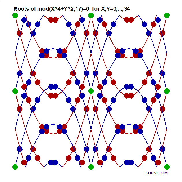
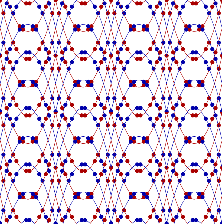
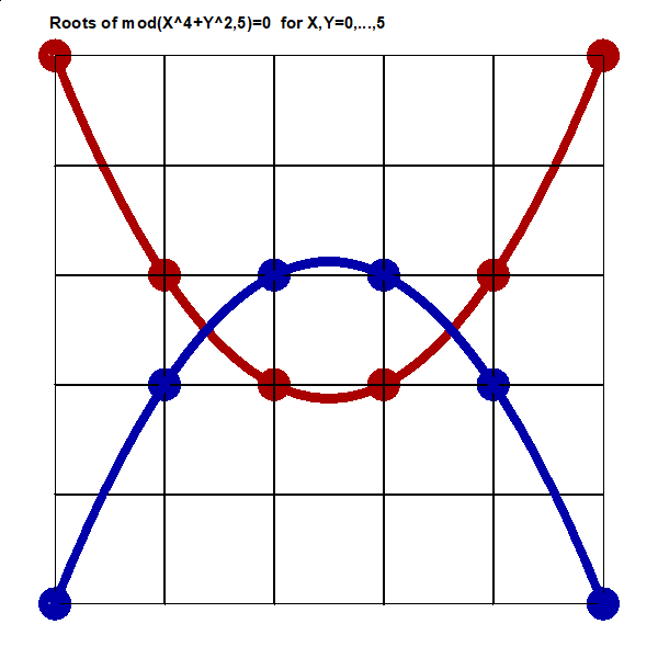
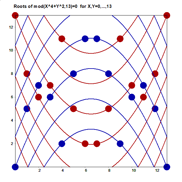
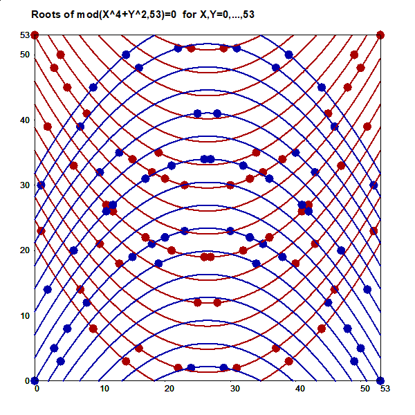
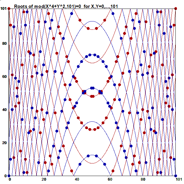
 11 *
 12 *TUTSAVE M
 13 *{tempo -1}{init}{jump 1,1,1,1}{erase}SCRATCH {home}{act}{line start}
 14 /
 15 *COLX W20{act}{line start}{erase}{tempo 2}{wait 50}{tempo -1}
 16 *{R}
 17 *   {form7} Roots of Diophantine equations mod(X^4+Y^2,P)=0 {R}
 18 *{R}
 19 *Diophantine equations of the form mod(X^4+Y^2,P)=0 have nontrivial{R}
 20 *solutions X,Y for primes P of the form P=4k+1.{R}
 21 *By making numerical experiments by means of Survo it is found that{R}
 22 *the roots X,Y for a given P are integer points on parabolas{R}
 23 *{R}
 24 *       Y=[+-(X^2-P*X)+P*i]/C(P){R}
 25 *{R}
 26 *where i is any integer and{R}
 27 *C(P) is the minimal integer square root of -1 modulo P.{R}
 28 *{R}
 29 *I have tested this result for the primes{R}
 30 *{R}
 31 *P     5,13,17,29,37,41,53,61,73   having the following C(P) values{R}
 32 *C(P)  2, 5, 4,12, 6, 9,23,11,27{R}
 33 *{R}
 34 *In this demo the case P=17 will be studied.
 35 *{tempo 2}{70}{R}{R}
 36 /
 37 *{tempo -1}{line start}
 38 *XSCALE=0,17  YSCALE=0,17 *GLOBAL*{R}
 39 *WSTYLE=0 HEADER=  XLABEL= YLABEL= XDIV=1,8,1 YDIV=1,8,1 FRAME=3{R}
 40 *WSIZE=990,990  WHOME=505,45 POINT=6,6 MODE=2000,2000{R}
 41 *....................................................{R}
 42 *{d23}{u21}{tempo 2}{10}
 43 /
 44 *The roots{tempo -1} of the equation mod(X^4+Y^2,17)=0 for X,Y<=17 are obtained{R}
 45 *by the Survo command (checking all X,Y combinations){R}
 46 *{l4}ab{r}{u2}
 47 /
 48 *DIOPH 4,2,17,17,CUR+4{tempo 2}{keys 2}{act}{keys 0}{10}
 49 /
 50 *{R}{R}
 51 *DATA K{R}
 52 *X  Y    C{20}{line start}{u2}
 53 /
 54 *GPLOT K,X,Y / WSIZE=630,630 WHOME=497,0 POINT=0,25
 55 *{keys 2}{act}{keys 0}{20}
 56 /
 57 *{home}{ins line}{ins line}{ins line}{ins line}{ins line}{ins line}
 58 *{ins line}{u5}{10}
 59 /
 60 *It is possible{tempo -1} to see{R}
 61 *that points may be{R}
 62 *located on a set{R}
 63 *of parabolas...{R}
 64 *{tempo +1}{30}
 65 /
 66 *{tempo -1}
 67 *{u}{erase}{u}{erase}{u}{erase}{u}{erase}/SOFT-PLOTCLS{act}{home}{erase}
 68 *{tempo 2}{10}
 69 /
 70 *For estimating{tempo -1} equations of these parabolas, the plot may be created{R}
 71 *so that each point is presented by its coordinates in the form x|y{R}
 72 *This is achieved as follows:{tempo 2}{30}
 73 *{R}{ref set 1}
 74 *{d4}{ins line}
 75 /
 76 *{tempo -1}{ref set 1}
 77 + A: {R}{next word}{save word W1}
 78 - if W1 '=' {sp} then goto B
 79 *{l}|{goto A}
 80 + B: {ref jump 1}{ref jump 1}{tempo +1}{10}
 81 /
 82 *I{l}{act}{act}{act}{act}{act}{act}{act}{act}{del line}{u3}{copy}a{R}
 83 *{r20}3{keys 2}{act}{keys 0}{R}
 84 *{u2}{copy}b{10}{R}
 85 *{r46}[CourierB(50)],C{keys 2}{act}{keys 0}{30}
 86 /
 87 *{home}{pre}{d}{pre}{d2}{10}
 88 /
 89 *Now following{tempo -1} points are{R}
 90 *on the same curve:{R}
 91 *DATA S:(X,Y) 7,8 10,8{R}
 92 *6,9 11,9 END{tempo +1}{R}
 93 /
 94 *{20}{tempo -1}/SOFT-PLOTCLS{tempo +1}{act}tempo -1}{home}{erase}
 95 *{tempo +1}{5}
 96 *{tempo -1}GPLOT FILE G{tempo +1}{act}{tempo -1}
 97 *{home}{erase}{tempo +1}{20}
 98 /
 99 *{tempo -1}/SOFT-PLOTCLS{act}{home}{erase}
100 *{R}
101 *{d16}{u16}{tempo 2}{15}
102 /
103 *Finding{tempo -1} the parabola going through those points by ESTIMATE operation:{R}
104 *{R}{tempo +1}
105 *MODEL M{R}
106 *Y=C*X^2+D*X+E{R}
107 *{R}
108 *ESTIMATE S,M,CUR+1 / RESULTS=0{10}{keys 2}{act}{keys 0}{20}
109 /
110 *{d2}{10}1/4{d}{l4}{10}-17/4{d}{l4}{10}3*17/2{10}{R}
111 *{R}
112 *{R}
113 *Then the formula of the parabola is{R}
114 *   {form}Y={form7}1/4*X^2-17/4*X+6*17/4{5}=(X^2-17*X+6*17)/4{5}={form}(X^2-P*X+6*P)/4 {form7}.
115 *{10}{R}
116 *Since the scatter plot{tempo -1} is symmetrical also{R}
117 *   {form}Y=(-X^2+P*X-6*P)/4{R}
118 *covers points in the graph.{tempo +1}{20}
119 /
120 *{d15}{u15}{R}{R}
121 *The complete set{tempo -1} of parabolas{R}
122 *covering all solutions{R}
123 *for X,Y=0,...,17{R}
124 *is obtained by plotting curves{R}
125 *   Y=(+X^2-P*X+i*P)/4, P=17{R}
126 *   Y=(-X^2+P*X-i*P)/4, i=-4(2)8{tempo +1}{30}{tempo -1}{R}
127 *{R}
128 *GPLOT FILE G42_17{act}{line start}{erase}{tempo +1}
129 *{end}
130 *
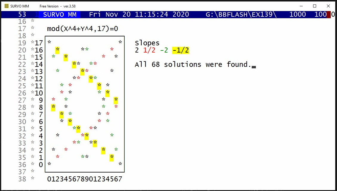
This demo in YouTube
The corresponding graph for n=2,P=5

   mod(X^2+Y^2,5)=0
    +------+
   5|*    *|
   4|  **  |
   3| *  * |
   2| *  * |
   1|  **  |
   0|*    *|
    +------+
     012345
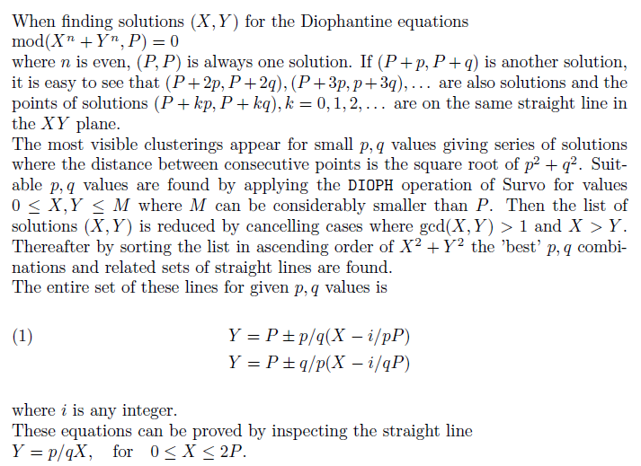
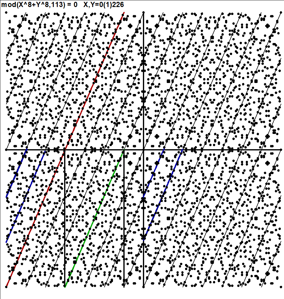
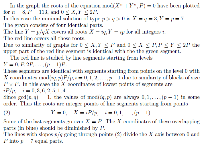
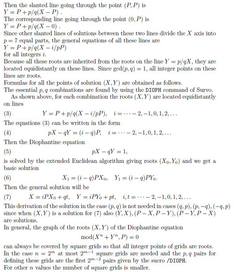
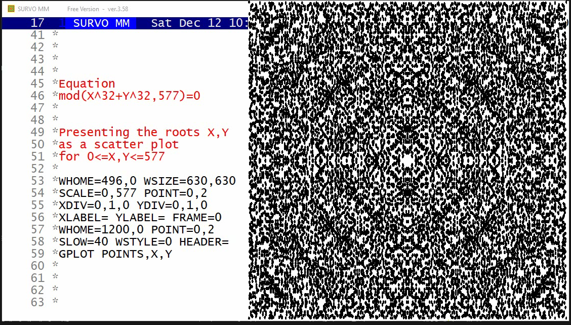
This demo in YouTube
It is possible to determine all roots of a Diophantine equation
X^n+Y^n ≡ 0 (mod P)
when n is an even integer and P is a prime
by simple arithmetical calculations (addition and subtraction)
after
the basic solutions, p,q integers close to zero are available.
In this process it is noticed that that each p,q pair gives the
same amount 4P of roots.
This is evident on the basis of the proof given in comments of the
preceding demo
Roots of mod(X^n+Y^n,P)=0 by simple arithmetics
In some cases the total number of roots is smaller due to overlapping.
However, the total number of solutions in the area 0<=X,Y<=P,
at least when n is a multiple of 4 and gcd(n,P-1)/4>=1,
is 4*(P-1)*N(n,P)+4 when the 4 trivial roots (0,0) (0,P) (P,0) (P,P)
are included.
N(n,P)=ceil[gcd(n,P-1)/4] is the number of starting points required,
but this has not been formally proved.
The starting points are the N(n,P) minimal solutions of mod(X^n+Y^n,P)=0
according to the distance from the origin.
It has been true in all cases presented in
# of roots and slopes in over 120 cases.
The new sucro /DI_SOLVE using a new Survo module DISOLVE finds
the correct p,q values and solutions for 0<=X,Y<=P.
The solutions are saved in a Survo data file POINTS containg values
of variables X,Y,C where C tells the relation to p,q combinations by
negative values -1,-2,...,-N(n,P).
At the end it is possible to check the result by activating
DIOPHF 32,32,577,577
which tests all X,Y combinations 0<=X,Y<=P and gives in this case
18436 as the total number of solutions.
Colored case n=100 P=401
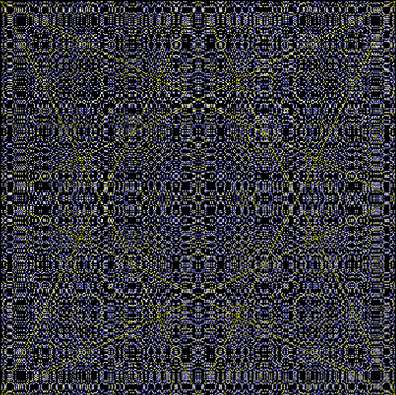
1600 points in each of 25 p,q combinations
This graph has been created by the following means in Survo:
 11 *
 12 */DI_SOLVE 100,100,401,100
 13 *DISOLVE 100,100,401,25
 14 *
 15 *  n   p   q   points
 16 *  1   1   2   1604
 17 *  2   2   5   1600
 18 *  3   1   7   1600
 19 *  4   1   8   1600
 20 *  5   4   7   1600
 21 *  6   5   7   1600
 22 *  7   1   9   1600
 23 *  8   5   8   1600
 24 *  9   4   9   1600
 25 * 10   1  10   1600
 26 * 11   5   9   1600
 27 * 12   1  11   1600
 28 * 13   4  11   1600
 29 * 14   5  11   1600
 30 * 15   3  13   1600
 31 * 16   9  14   1600
 32 * 17   3  17   1600
 33 * 18   7  16   1600
 34 * 19  12  13   1600
 35 * 20  11  14   1600
 36 * 21   9  16   1600
 37 * 22   3  19   1600
 38 * 23   7  18   1600
 39 * 24  11  16   1600
 40 * 25  13  15   1600
 41 *
 42 *npq=25 n_total=40004 P=401
 43 *n_total=40004 is equal to 4*npq*(P-1)+4=40004
 44 *
 45 *FILE SAVE POINTS.TXT TO NEW POINTS
 46 *FILE DEL POINTS.TXT
 47 *FILE SHOW POINTS
 48 *Check results by activating:
 49 *DIOPHF 100,100,401,401
 50 *n=40004
 51 *
 52 *>REN POINTS.SVO P100_401.SVO
 53 *FILE SHOW P100_401
 54 *......................................
 55 *
 56 *WSTYLE=0 HEADER=  XLABEL= YLABEL= XDIV=0,1,0 YDIV=0,802,40 FRAME=3
 57 *WSIZE=802,842 WHOME=900,0 MODE=2000,2000 TEXTS=T
 58 *XSCALE=-1,400 YSCALE=0,400
 59 *T=[SwissB(40)][WHITE],mod(X^100+Y^100;401)_=_0___X;Y=0(1)401,100,1925
 60 *GPLOT P100_401,X,Y  / SLOW=50 WSTYLE=0
 61 *FILE SHOW P100_401
 62 *FRAME=0                      PEN=[BLACK]
 63 *POINT=0,3   POINT_COLOR=C    COLORS=[BLACK][/BLACK]
 64 *
 65 * FILL(-1)=0,0,1,0
 66 * FILL(-2)=0.5,0.5,0,0
 67 * FILL(-3)=0,0,1,0
 68 * FILL(-4)=0.5,0.5,0,0
 69 * FILL(-5)=0,0,1,0
 70 * FILL(-6)=0.5,0.5,0,0
 71 * FILL(-7)=0,0,1,0
 72 * FILL(-8)=0.5,0.5,0,0
 73 * FILL(-9)=0,0.0,0.0,0
 74 *FILL(-10)=0.5,0.5,0,0
 75 *FILL(-11)=0,0.0,0.0,0
 76 *FILL(-12)=0.5,0.5,0,0
 77 *FILL(-13)=0,0.0,0.0,0
 78 *FILL(-14)=0.5,0.5,0,0
 79 *FILL(-15)=0,0.0,0.0,0
 80 *FILL(-16)=0.5,0.5,0,0
 81 *FILL(-17)=0,0.0,0.0,0
 82 *FILL(-18)=0.5,0.5,0,0
 83 *FILL(-19)=0,0.0,0.0,0
 84 *FILL(-20)=0.5,0.5,0,0
 85 *FILL(-21)=0,0.0,0.0,0
 86 *FILL(-22)=0.5,0.5,0,0
 87 *FILL(-23)=0,0.0,0.0,0
 88 *FILL(-24)=0.5,0.5,0,0
 89 *FILL(-25)=0,0.0,0.0,0
 90 *
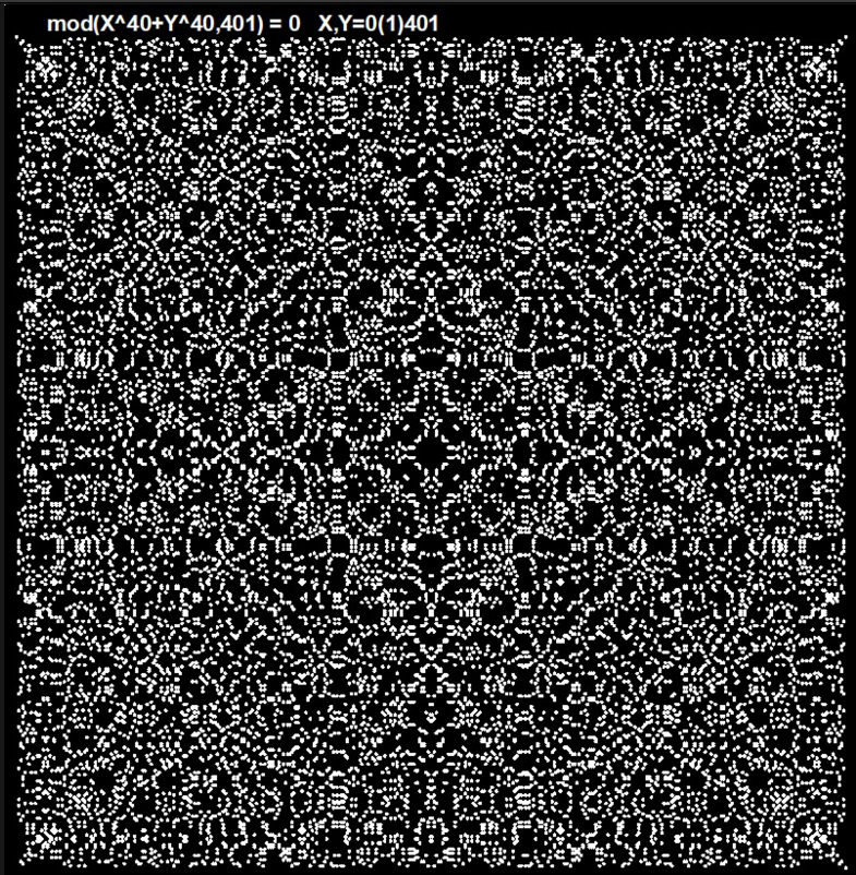
This demo in YouTube
The roots of Diophantine equations X^n+Y^n ≡ 0 (mod P)
can be determined by using simple arithmetics as shown in 2 previous
demos
Roots of mod(X^n+Y^n,P)=0 by simple arithmetics
Roots of mod(X^n+Y^n,P)=0 by simple arithmetics 2
In earlier demos the roots were presented from the middle of the graph
towards borders.
In this demo the roots emerge from corners towards the center
according to that simple arithmetics.
As shown in preceding demos, the roots of Diophantine equations X^n+Y^n ≡ 0 (mod P)
in the ares 0<=X,Y<=P are found when P is a prime number and
n is an even integer as follows:
At first GCD(n,P-1)/4 minimal roots X,Y are found by inspecting
points (X,Y) close to the origin (0,0).
For each of them related roots are found by projecting roots
(kX,kY), k=1,2,... to the area 0<=X,Y<=P and using the rules:
If (X,Y) is a root, then also
(Y,X), (P-X,Y), (P-Y,X), (X,P-Y), (P-X,Y), (P-X,P-Y), (P-Y,P-X) are roots.
Giving the same color in the graph for all roots related
to the same minimal root emphasizes the structure of the entire solution.
Mathematical background information
More demos of the same type:
Demo 2: YouTube
Demo 3: YouTube
New summary (7 October 2022)
Seppo Mustonen: Additional results on the roots of nonlinear Diophantic equations mod(X^n+Y^n,P)=0 (2022)
Earlier summary
Seppo Mustonen: On the roots of nonlinear Diophantic equations mod(X^n+Y^n,P)=0 (2018)
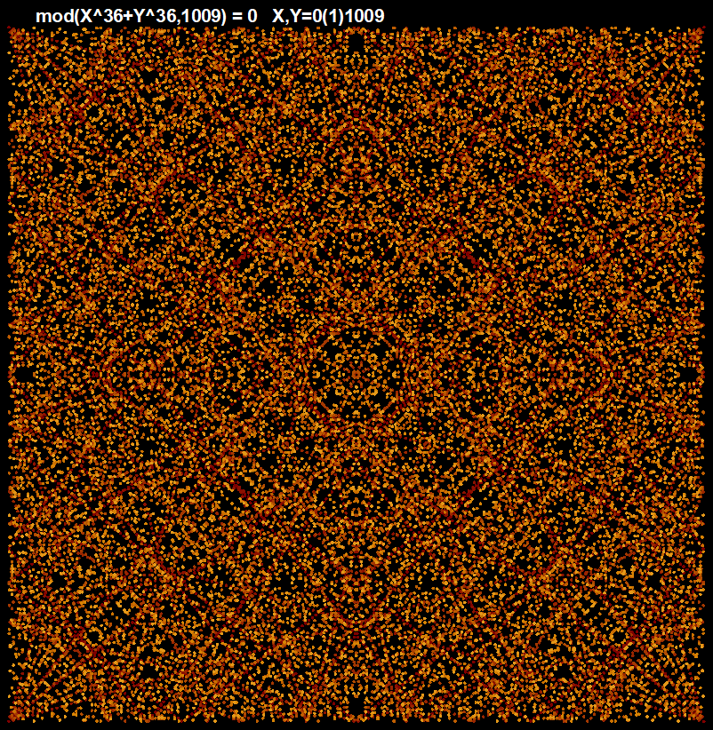
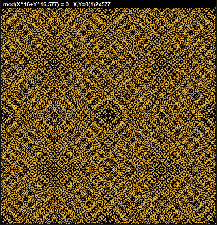
This demo in YouTube
Twelve graphs given earlier in
Automatic solution of nonlinear Diophantine equations mod(X^n+Y^n,P)=0
as monochrome static printouts are now displayed in a dynamic and colored form.
Information about creation of these graphs is given in
Technical background information
Seppo Mustonen: On the roots of nonlinear Diophantic equations mod(X^n+Y^n,P)=0 (2018)
The final forms of these 12 dynamic graphs:
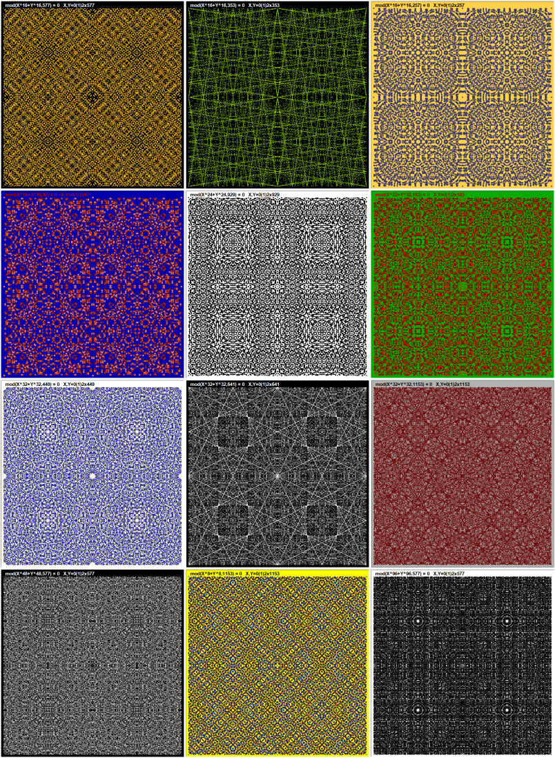
Some intermediate stages of the last case mod(X^96+Y^96,577)=0
Video in YouTube
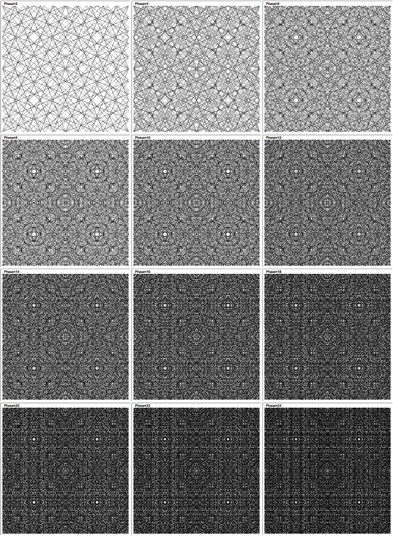
Some intermediate stages of the fifth case mod(X^24+Y^24,929)=0
Video in YouTube
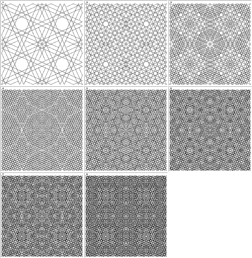
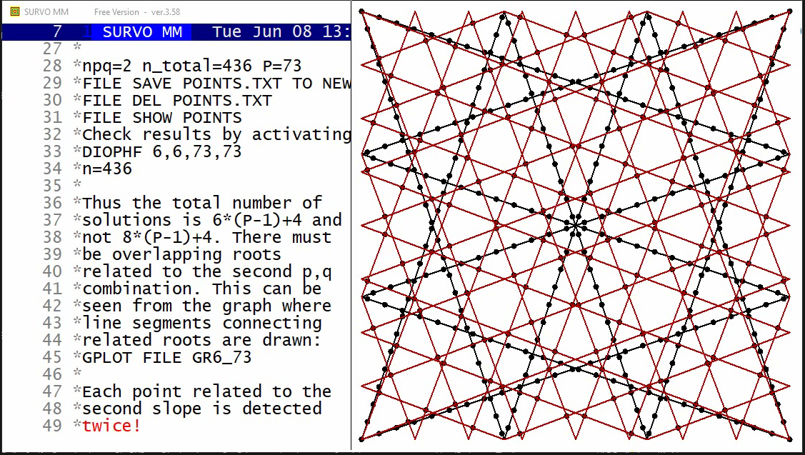
New demo in YouTube
When n is a multiple of 4 and P is a prime number
it is evident that the number of square grids
covering all roots of the Diophantine equation mod(X^n+Y^n,P)=0
is GCD(n,P-1)/2 (2 grids for each p,q combination)
Since each square grid depends on two parameters determining its
slope, the entire solution depends on GCD(n,P-1) slope parameters.
This interpretation can be extended to the case where n is even
and not necessarily a multiple of 4.
Then it is evident that when n is even, the number of slopes needed
for straight lines covering all roots is also GCD(n,P-1).
As an example the case n=6, P=73 where GCD(n,P-1)=6 is studied.
In this case two p,q combinations (1,3) and (3,8) are obtained.
giving 8 possible directions, but two of the (3,8) combinations
give the same solutions twice so that the roots are located
on the crossing points of the slanted grid defined by the combination
(3,8) as one can see in the graph above.
In this case the 6 slopes are 1/3, -1/3, 3/1, -3/1, 3/8, 8/3.
The following excerpt from the demo tells about these results:
Finding p,q values and number of solutions for each combination:
/DI_SOLVE 6,6,73,100
DISOLVE 6,6,73,2

  n   p   q   points
  1   1   3    292 4*(P-1)+4=292
  2   3   8    144 2*(P-1)=144

npq=2 n_total=436 P=73
FILE SAVE POINTS.TXT TO NEW POINTS / Activate!
FILE DEL POINTS.TXT                / Activate!
FILE SHOW POINTS
Check results by activating:
DIOPHF 6,6,73,73
n=436
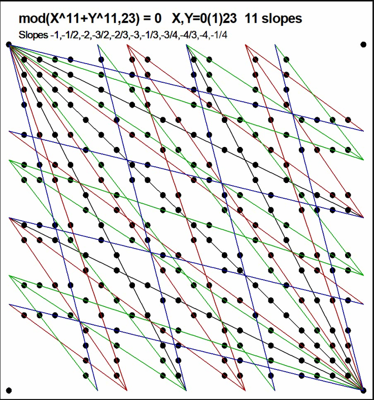
This demo in YouTube
As shown in the graph above the roots of the Diophantine equation
mod(X^11+Y^11,23)=0 for 0 ≤ X,Y ≤ 23 are located on straight lines with
GCD(11,23-1)=11 different slopes.
Each nontrivial root is covered by a single line.
Roots on each line are located equidistantly.
The same pattern of roots can be extended to any direction by steps n=23.
In general it is obvious that also when n is an odd integer the
number of slopes needed for straight lines to cover all roots
of Diophantine equations mod(X^n+Y^n,P)=0 when P is a prime number
is GCD(n,P-1).
This result has been indicated the earlier demo
Number of slopes for lines covering roots of mod(X^n+Y^n,P)=0
for even integers n.
In all cases the roots are the integer points on these lines.
On the basis of results obtained in these demos my general hypothesis is:
When P is a prime and n is a positive integer,
the roots of Diophantine equations mod(X^n+Y^n,P)=0
are equidistantly on straight lines with GCD(P-1,n) possible slopes
determined by roots (X,Y) closest to (0,0).
Besides trivial roots with coordinates as multiples of P,
each root is located on only one of those lines and
all integer points on those lines are roots.
So far only a limited number of odd cases have been tested.
 n   P   GCD(n,P-1)   Slopes
 3  19    3           -1 -(2,3)
 3  31    3           -1 -(1,5)
 3  37    3           -1 -(3,4)
 3  43    3           -1 -(1,6)
 3  61    3           -1 -(4,5)
 3  67    3           -1 -(2,7)
 3  73    3           -1 -(1,8)
 3  79    3           -1 -(3,7)
 3 103    3           -1 -(2,9)
 3 109    3           -1 -(5,7)
 3 127    3           -1 -(6,7)
 3 139    3           -1 -(3,10)
 5  11    5           -1 -(1,3) +(1,2)
 5  31    5           -1 -(1,2) -(1,4) or
 5  31    5           -1 -(1,2) +(3,7)
 5  41    5           -1 -(3,7) +(1,4)
 5  61    5           -1 -(2,7) +(1,3)
 5  71    5           -1 -(3,4) +(1,14)
 5 101    5           -1 -(3,7) +(1,6)
 5 131    5           -1 -(1,3) +(2,9)
 7  29    7           -1 -(2,3) -(4,5) -(1,7)
 7  43    7           -1 -(1,4) -(3,5) +(1,2)
 7  71    7           -1 -(2,3) -(4,9) +(3,7)
 7 113    7           -1 -(4,7) +(1,4) +(1,7)
 7 127    7           -1 -(1,2) -(1,4) +(7,15)
 9  13    3           -1 -(1,3)
 9  37    9           -1 -(3,4) -(5,8) -(1,7) -(1,12)
11  23   11           -1 -(1,2) -(1,3) -(2,3) -(3,4) -(1,4)
11  67   11           -1 -(3,5) -(3,8) -(5,8) +(1,3) +(1,5)
13  53   13           -1 -(2,3) -(6,7) -(4,7) -(4,9) -(7,11) -(9,11)
15  31   15           -1 -(1,2) -(4,5) -(2,5) -(1,4) -(4,7) -(5,7) -(1,10)
17 103   17           -1 -(4,7) -(1,8) -(3,10) -(5,11) -(8,9) -(5,12) +(1,3) +(4,5)
19 191   19           -1 -(1,5) -(1,6) -(5,6) -(8,9) -(8,13) -(9,13) +(3,7) +(1,11) +(5,11)
21  29    7           -1 -(2,3) -(1,7) +(1,5)
21  43   21           -1 -(2,3) -(1,4) -(2,5) -(3,5) -(1,6) -(2,7) -(3,8) -(5,7) +(1,2) +(1,3)
23  47   23           -1 -(1,2) -(1,3) -(2,3) -(1,4) -(3,4) -(1,6) +(1,5) +(2,5) +(3,5) +(4,5) +(5,6)
25  31    5           -1 -(1,2) -(1,4)
27  19    9           -1 -(2,3) -(1,4) +(1,2) +(1,3)
29  59   29           -1 -(1,3) -(1,4) -(4/3) -(5,3) -(1,5) -(1,7) -(1,9) +(2,1) +(3,2) +(5,2) +(6,1) +(7,2) +(7,6) +(8,1)
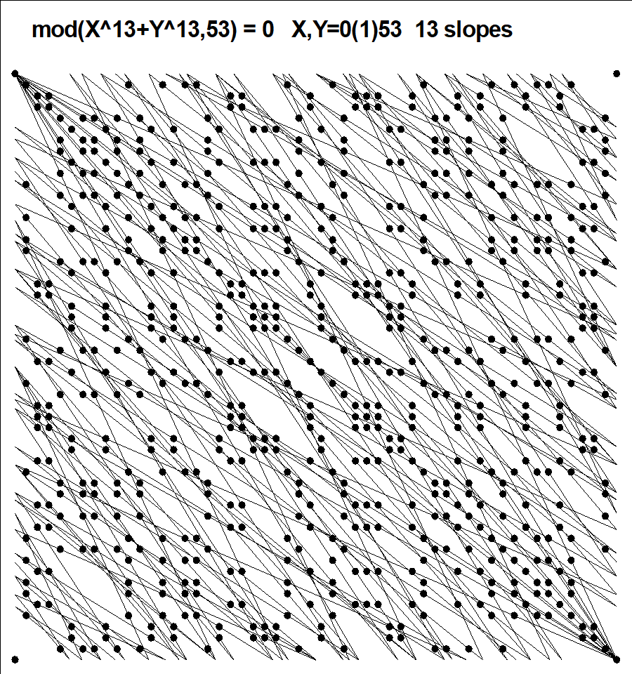
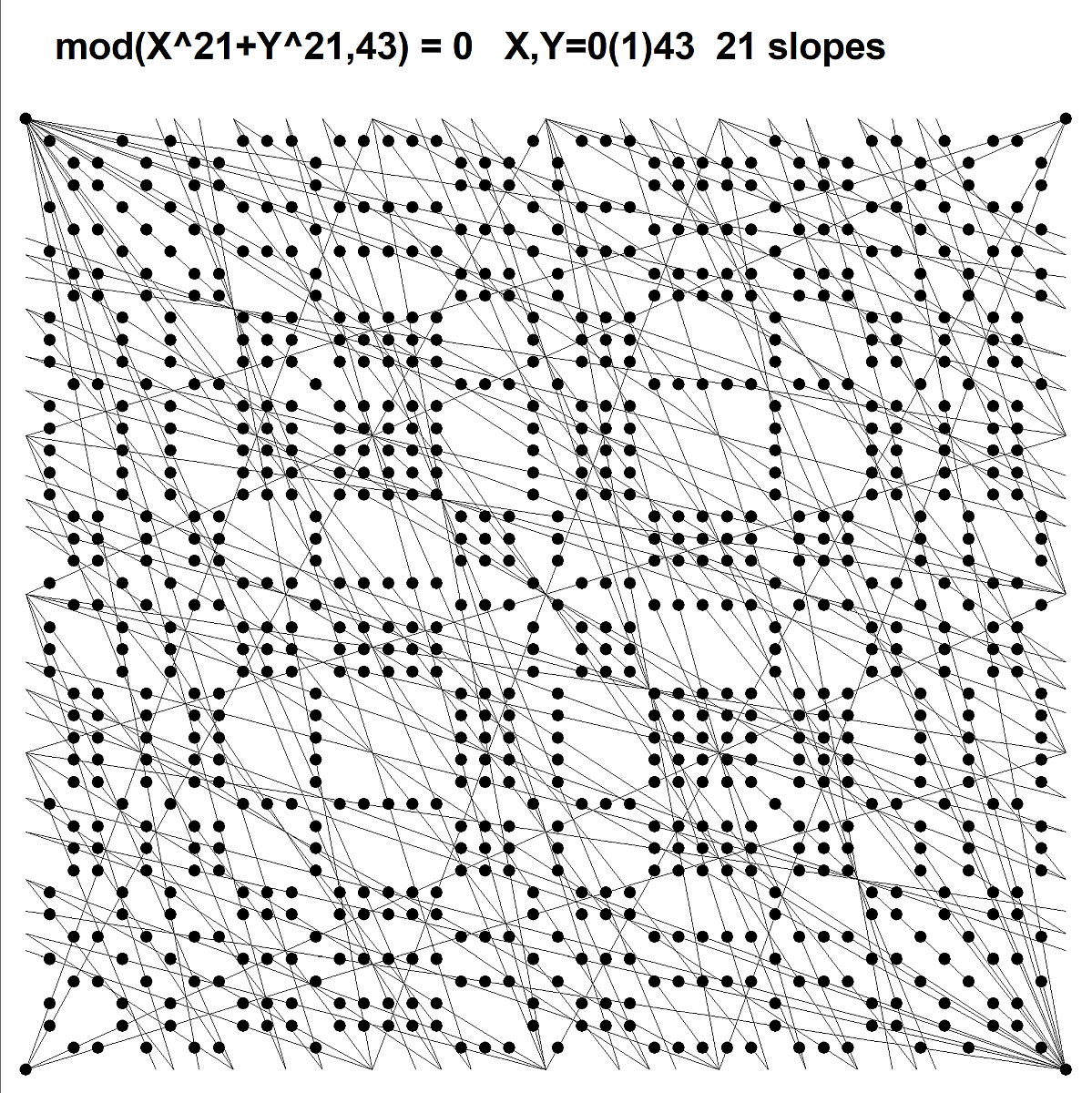
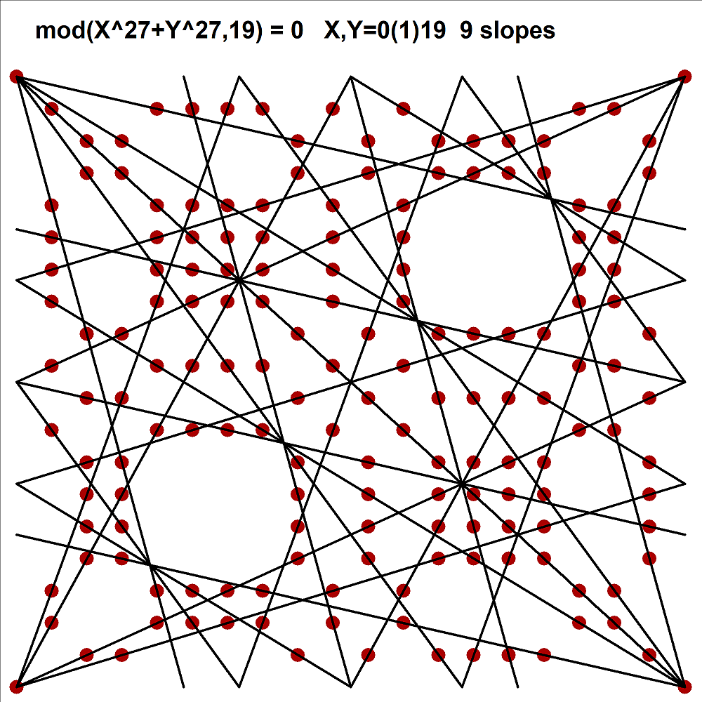
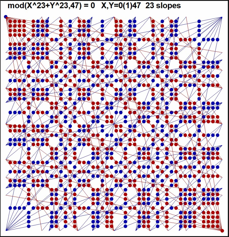
This demo in YouTube
The roots of mod(X^n+Y^n,P)=0 for n=23, P=47 are plotted stepwise
by starting from GCD(P-1,n)=23 minimal roots
(-1,-1)
(-1,2) (-1,3) (-2,3) (-1,4) (-3,4) (-1,6) (1,5) (2,5) (3,5) (4,5) (5,6)
(-2,1) (-3,1) (-3,2) (-4,1) (-4,3) (-6,1) (5,1) (5,2) (5,3) (5,4) (6,5).
in the area 0<=X,Y<=47.
Calculations of coordinates for the multiples of these basic roots
were performed modulo P until a point in the corner of
the area 0<=X,Y<=P was reached.
The roots related to descending slopes are red and ascending ones
are blue.
At the end the straight lines covering the roots are drawn.
Each root (except those in corners) is located on only one of these lines.
The number of slopes of the lines is GCD(P-1,n)=23.
In all directions P-1 nontrivial solutions were found.
It is obvious that when n is odd and GCD(P-1,n)>0,
GCD(P-1,n)*(P-1) roots for 0 < X,Y < P are found.
In this case we got GCD(P-1,n)*(P-1)+4=1062 roots.
New demo in YouTube
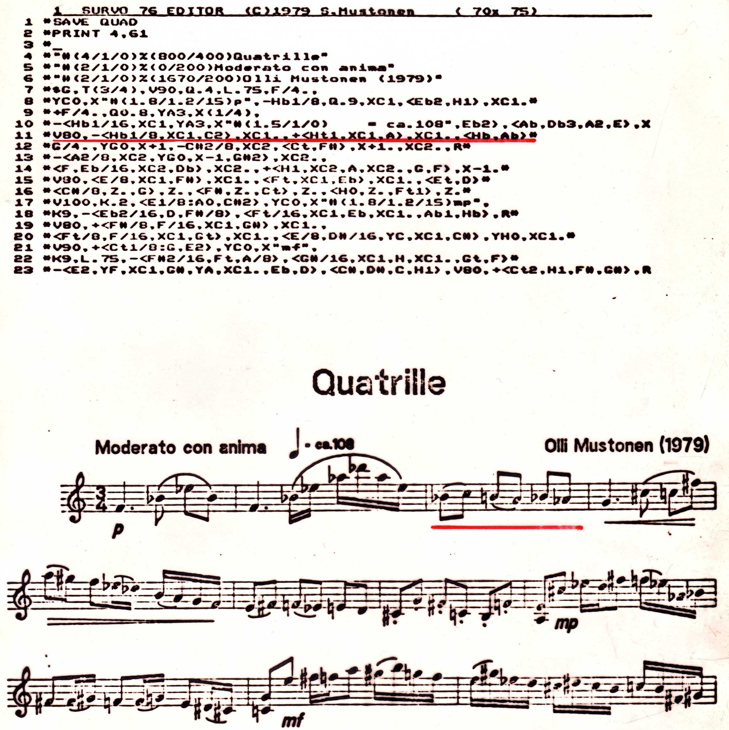
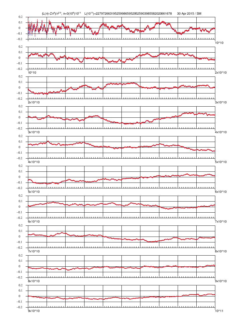
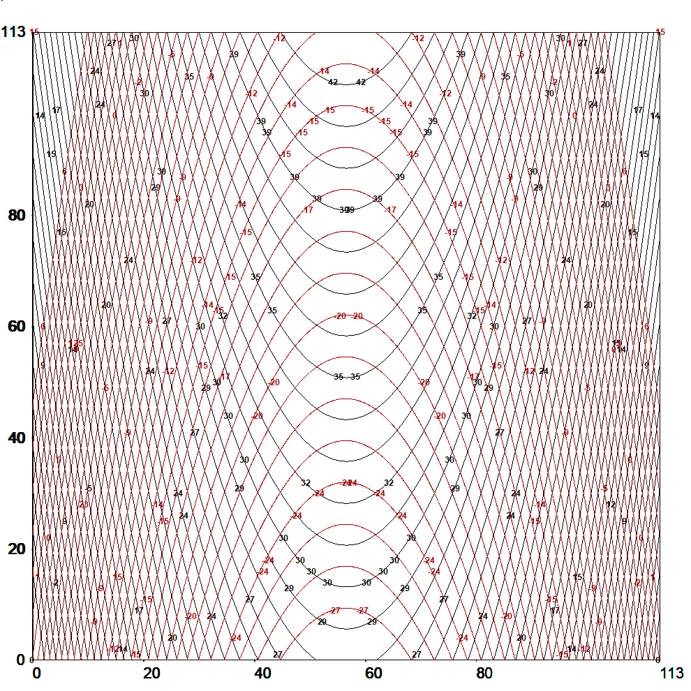