The Eighth International Workshop on Matrices and Statistics

Matrix computations in Survo

Introduction

Survo is a general environment for statistical computing and related areas (Mustonen 1992). Its current version SURVO 98 works on standard PC's and it can be used in Windows, for example. The first versions of Survo were created already in 1960's. The current version is based on principles introduced in 1979 (Mustonen 1980, 1982).
     According to these principles, all tasks in Survo are handled by a general text editor. Thus the user types text and numbers in an edit field which is a rectangular working area always partially visible in a window on the computer screen. Information from other sources - like arrays of numbers or textual paragraphs - can also be transported to the edit field.
     Although edit fields can be very large giving space for big matrices and data sets, it is typical that such items are kept as separate objects in their own files in compressed form and they are referred to by their names from the edit field. Data and text are processed by activating various commands which may be typed on any line in the edit field. The results of these commands appear in selected places in the edit field and/or in output files. Each piece of results can be modified and used as input for new commands and operations.
     This interplay between the user and the computer is called `working in editorial mode'. Since everything is directly based on text processing, it is easy to create work schemes with plenty of descriptions and comments within commands, data, and results. When used properly, Survo automatically makes a readable document about everything which is done in one particular edit field or in a set of edit fields. Edit fields can be easily saved and recalled for subsequent processing.
     Survo provides also tools for making new application programs. Tutorial mode permits recording of Survo sessions as sucros (Survo macros). A special sucro language for writing sucros for teaching and expert applications is available. For example, it is possible to pack a lengthy series of matrix and statistical operations with explanatory texts in one sucro. Thus stories about how to make statistical analysis consisting of several steps can be easily told by this technique. Similarly application programs about various topics are created rapidly as sucros.
     Matrix computations are carried out by the matrix interpreter of Survo (originated in its current form in 1984 and continuously extended since then). Each matrix is stored in its own matrix file and matrices are referred to by their file names. A matrix in Survo is an object having five attributes:

1. Internal name of matrix, for example, INV(X'*X)*X'*Y,
2. # of rows and columns,
3. Type of matrix (general, symmetric, diagonal),
4. Labels of rows and columns, each up to 8 characters,
5. Matrix elements, real numbers in double precision.

A matrix has always an internal name, typically a matrix expression that tells the `history' of the matrix. The internal name is formed automatically according to matrix operations which have been used for computing this particular matrix. Also row and column labels - extremely valuable for identifying the elements - are inherited in a natural way. Thus when a matrix is transposed or inverted, row and column labels are interchanged by the Survo matrix interpreter. Such conventions guarantee that resulting matrices have names and labels reflecting the true role of each element. Assume, for example, that for linear regression analysis we have formed a column vector Y of values of regressand and a matrix X of regressors. Then the command

MAT B=INV(X'*X)*X'*Y

gives the vector of regression coefficients as a column vector (matrix file) B with internal name INV(X'*X)*X'*Y and with row labels which identify regressors and a (single) column label which is the name of the regressand. The following small example illustrates these features.

14 1 SURVO 98 Sun Jul 04 17:22:19 1999 D:\TRE\ 1000 100 0

1 *SAVE STAT12 / International statistics (Source: Statistics Finland) 2 * 3 *Variables: 4 *Life Life expectancy in years, 1997 5 *GDP Gross Domestic Product per Capita (US $), 1997 6 *Growth Population Growth, %/year, 1996-1997 7 * 8 *MATRIX WORLD12 9 * /// Life GDP Growth Constant 10 * China 70 0.860 1.0 1 11 * Finland 77 24.790 0.3 1 12 * France 78 26.300 0.4 1 13 * Hungary 71 4.510 -0.4 1 14 * Japan 80 38.160 0.3 1 15 * Mexico 72 3.700 1.7 1 16 * Nigeria 54 0.280 2.9 1 17 * Romania 69 1.410 -0.2 1 18 * Sweden 79 26.210 0.1 1 19 * Turkey 69 3.130 1.7 1 20 * UK 77 20.870 0.4 1 21 * USA 76 29.080 0.9 1 22 * 23 *MAT SAVE WORLD12 24 *MAT Y!=WORLD12(*,Life) 25 *MAT X!=WORLD12(*,GDP:Constant) 26 * 27 *MAT B=INV(X'*X)*X'*Y 28 *MAT LOAD B_ 29 *MATRIX B 30 *INV(X'*X)*X'*Y 31 */// Life 32 *GDP 0.3078 33 *Growth -3.4502 34 *Constant 70.6838 35 *

Comments:
Above a part of the current edit field is shown as it appears in a window during a Survo session. The activated Survo commands appear (just for illustration here) in inverse mode and results given by Survo on a gray background.

A small table of data values (loaded to the edit field from a larger data file) is located on edit lines 8-21. It is labelled as a matrix WORLD12 (line 8). The data set is saved in a matrix file WORLD12 by activating the MAT SAVE command on line 23. The vector of dependent variable Life is extracted from WORLD12 by the command MAT Y!=WORLD12(*,Life). The `!' character indicates that Y will be also the internal name of matrix file Y. Similarly the matrix of independent variables is saved as a matrix file X (line 25). The regression coefficients are computed by the command on line 27 and loaded into the edit field by the MAT LOAD command on line 28.

Various statistics related to a linear regression model can be calculated according to standard formulas as follows:

14 1 SURVO 98 Mon Jul 05 08:59:23 1999 D:\TRE\ 1000 100 0

35 * 36 *n=12 k=2 Number of cases and independent variables 37 *Residual sum of squares: 38 *MAT SSE=Y'*(IDN(n,n)-X*INV(X'*X)*X')*Y 39 *Residual mean square: 40 *MAT MSE=SSE/(n-k-1) / *MSE~Y'*(IDN-X*INV(X'*X)*X')*Y/(n-k-1) D1*1 41 *MAT_MSE(1,1)=13.046466274137 42 * 43 *Total sum of squares: 44 *MAT J1=CON(n,1) 45 *MAT J=J1*J1'/n 46 *MAT SST=Y'*(IDN(n,n)-J)*Y 47 * 48 *Multiple correlation coefficient squared: 49 *R2=1-MAT_SSE(1,1)/MAT_SST(1,1) 50 *R2=0.7890691081427 51 * 52 *Estimated covariance matrix of regression coefficients: 53 *MAT COV_B=MSE*INV(X'*X) 54 *MAT LOAD COV_B 55 *MATRIX COV_B 56 *Y'*(IDN-X*INV(X'*X)*X')*Y/(n-k-1)*INV(X'*X) 57 */// GDP Growth Constant 58 *GDP 0.00744 0.04419 -0.14474 59 *Growth 0.04419 1.59233 -1.86776 60 *Constant -0.14474 -1.86776 4.66623 61 * 62 *Estimated standard deviations of regression coefficients: 63 *MAT SD_B=VD(DIAG(COV_B)^0.5) 64 *MAT LOAD SD_B_ 65 *MATRIX SD_B 66 *VD(DIAG(Y'*(IDN-X*INV(X'*X)*X')*Y/(n-k-1)*INV(X'*X))^0.5) 67 */// diag 68 *GDP 0.086280 69 *Growth 1.261874 70 *Constant 2.160146 71 *

The computations like those above are suitable in teaching but not efficient enough for large scale applications. Of course Survo provides several means for direct calculations of linear regression analysis. For example, the REGDIAG operation based on the QR factorization of X gives in its simplest form the following results:

26 1 SURVO 98 Mon Jul 05 09:22:01 1999 D:\TRE\ 1000 100 0

72 *....................................................................... 73 *VARS=Life(Y),GDP(X),Growth(X) 74 *REGDIAG WORLD12.MAT,CUR+1_ 75 *Regression diagnostics on data WORLD12.MAT: N=12 76 *Regressand Life # of regressors=3 (Constant term included) 77 *Condition number of scaled X: k=3.92304 78 *Variable Regr.coeff. Std.dev. t 79 *Constant 70.683786 2.1601464 32.722 80 *GDP 0.3078164 0.0862801 3.5676 81 *Growth -3.4502111 1.2618736 -2.7342 82 *Variance of regressand Life=50.60606061 df=11 83 *Residual variance=13.04646627 df=9 84 *R=0.8883 R^2=0.7891 Durbin-Watson=2.380 85 *

All statistical operations of Survo related e.g. to linear models and multivariate analysis give their results both in legible form in the edit field and as matrix files with predetermined names. Then it is possible to continue calculations from these matrices by means of the matrix interpreter and form additional results. When teaching statistical methods it is illuminating to use the matrix interpreter for displaying various details step by step.

Typical statistical systems (like SAS, SPSS, S-Plus) as well as systems for symbolic and/or numerical computing (like Mathematica, Maple V, Matlab) include matrix operations as an essential part. There is, however, variation in how well these operations are linked to the other functions of the system. As far as I know those systems do not provide natural ways for keeping track on matrix labels and expressions in the sense described above.
     In statistical systems we usually have symbolic labels for variables and observations and these labels appear properly in tables of results. However, when data or results from statistical operations are treated by matrix operations, those labels are discarded. Thus when studying a resulting matrix it is often impossible to know what is its meaning or substance without remembering all the preceding operations which have produced it.
     In these circumstances one of the targets of this paper is to show the importance and benefits of automatic labelling in matrix computations by examples done in Survo. Another goal is to demonstrate the interface typical for Survo and co-operation of a statistical system and its matrix interpreter. Such important aspects as accuracy, speed, and other self-evident qualities of numerical algorithms have a minor role in this presentation.
     The main example used for describing the capabilities of the matrix interpreter deals with a certain subset selection problem. It is quite possible that this problem has been solved in many ways earlier. So far, however, I have not found any sources of similar attempts. In any case, in this context it is sufficient that this problem gives several opportunities to show how the matrix interpreter and Survo in general can be employed in research work.

Column space

Some months before this workshop Simo Puntanen asked me to implement computation of the basis of the column space of a given mxn matrix A as a new operation in Survo. When the rank of A is r, this space should be presented as a full-rank mxr matrix B. I answered by suggesting two alternative solutions. Both of them are based on the SVD of A since singular values provide a reliable basis for rank determination which may be a tricky task in the presence of roundoff (Golub and Van Loan, 1989, p.245-6).
     If the SVD of A is A = UDV^T, the simplest solution is to select B = U₁ where U₁ is formed of the r first columns of U. I felt, however, that in certain applications it would be nice to stick to a `representative' subset of columns of A although such a basis is not orthogonal in a general case. In particular when A is a statistical data matrix, it is profitable to eliminate superfluous variables which cause multicollinearity. The problem is now, how to select the `best' subset of r columns from n possible ones.
     There are plenty of books and papers about subset selection, for example, in regression analysis, but I think that it is another problem due to presence of a regressand or dependent variable or other external information.
     With my colleagues I had encountered a similar problem in connection of factor analysis when searching for a good oblique rotation in early 1960's. Our solution was never published as a paper. It has existed only as an algorithm implemented in Survo.

This approach when applied to the present task is to find a maximally orthogonal subset. One way to measure the orthogonality of a set of vectors is to standardize each of them to unit length and compute the volume of the simplex spanned by these unit vectors. Thus we could try to maximize the rxr major determinant of the nxn matrix of cosines of the angles between columns of A. When n and r are large, the total number of alternatives C(n,r) is huge and it is not possible to scan through all combinations. Fortunately there is a simple stepwise procedure which (crudely described) goes as follows:

det = 0
for i = 1:n 
     k(1) = i 
     for j = 1:r 
          det1 = 0
          for h = 1:n  
               det2 = determinant_of_cosines_from(A(k(1)), ..., A(k(j - 1)), A(h))
               if |det2| > det1
                    det1 = |det2| 
                    k(j) = h 
               end 
          end 
     end 
     if det1 > det 
          det = det1
          for j = 1:r      
               s(j) = k(j)
          end 
     end 
end 

In this stepwise procedure each column in turn is taken as the first vector and partners to this first one are sought by requiring maximal orthogonality in each step. Thus when j (j = 1, ..., r - 1) columns have been selected, the (j + 1)'th one will the column which is as orthogonal as possible to the subspace spanned by the j previous columns. From these n stepwise selections naturally the one giving the maximum volume (determinant value) is the final choice.
     To gain optimal performance the determinants occuring in this algorithm are also to be computed stepwise.
     It is not guaranteed that A(s(1)), ..., A(s(r)) is the best selection among all C(n,r), but according to my experience (see notes below) it is always reasonably close to the `best' one.

The determinant criterion is, of course, only one possible measure for orthogonality. In many statistical applications it corresponds to the generalized variance - determinant of the covariance matrix - which has certain weaknesses as a measure of total variability (see e.g. Kowal 1971, Mustonen 1997) but those are not critical in this context.
     Another alternative could be the condition number of the columnwise normalized matrix, but since it depends on the singular values, it seems to be too heavy at least computationally.
     The QR factorization with column pivoting and a refined form of it based on the SVD as suggested by Golub and Van Loan (1989, p.572-) for finding a "sufficiently independent subset" is an interesting alternative. At least the QR technique might be closely related to the determinant criterion, but so far I have had not time for comparisons.

The next numerical example illustrates how Survo is used for calculations of the column space.

1 1 SURVO 98 Mon Jul 05 11:22:04 1999 D:\TRE\ 1000 100 0

1 *SAVE COLSPACE 2 * 3 *In the following example the column space of a 8*7 matrix A 4 *is found by using the matrix interpreter (MAT commands) of 5 *the current version of SURVO 98. 6 *All text here is presented as such in the edit field of Survo. 7 * 8 *Matrix A with row and column labels is entered as follows: 9 *MATRIX A 10 */// C1 C2 C3 Sum1 C5 C6 Sum2 11 *R1 3 4 -1 6 2 -3 -1 12 *R2 5 2 3 10 5 5 10 13 *R3 0 -6 7 1 0 0 0 14 *R4 3 3 3 9 3 1 4 15 *R5 5 -2 4 7 1 7 8 16 *R6 3 0 0 3 2 -6 -4 17 *R7 1 2 3 6 3 8 11 18 *R8 8 1 -5 4 4 0 4 19 * 20 *In this case there are two trivial linear dependencies between columns, 21 *Sum1=C1+C2+C3 and Sum2=C5+C6. Of course, the matrix interpreter 22 *only carries the labels logically through calculations, but does not 23 *`see' that columns `Sum1' and `Sum2' are possible sums of certain 24 *other columns. 25 * 26 *By activating the following line, matrix A is saved in a matrix file: 27 *MAT SAVE A 28 *Singular value decomposition of A is computed by the next command: 29 *MAT SVD OF A TO U,D,V 30 *The diagonal matrix of singular values is presented as a column vector 31 *and loaded into the edit field by the command: 32 *MAT LOAD D,12.123456789012345,CUR+1 33 *MATRIX D 34 *Dsvd(A) 35 */// sing.val 36 *svd1 29.268814299847410 37 *svd2 14.862063607353040 38 *svd3 10.441562474137190 39 *svd4 7.280498647225781 40 *svd5 2.902358929986689 41 *svd6 0.000000000000001 42 *svd7 0.000000000000001 43 * 44 *Obviously rank(A) is 5 and the two last columns of V clearly reveal 45 *the dependencies between columns: 46 *MAT LOAD V(*,6:7) 47 *MATRIX V 48 *Vsvd(A) 49 */// svd6 svd7 50 *C1 0.00000 -0.50000 51 *C2 0.00000 -0.50000 52 *C3 0.00000 -0.50000 53 *Sum1 0.00000 0.50000 54 *C5 0.57735 0.00000 55 *C6 0.57735 0.00000 56 *Sum2 -0.57735 0.00000 57 * 58 *An orthonormal basis for the column space of A is given by 59 *MAT U1!=U(*,1:5) 60 *MAT LOAD U1 61 *MATRIX U1 62 */// svd1 svd2 svd3 svd4 svd5 63 *R1 -0.11540 0.50599 -0.12033 -0.32924 -0.29185 64 *R2 -0.57760 0.06298 -0.03419 -0.07066 0.33295 65 *R3 -0.04171 -0.29609 -0.74184 0.29013 0.28495 66 *R4 -0.35314 0.22788 -0.25609 -0.39832 -0.12640 67 *R5 -0.46266 -0.22590 -0.14785 0.35454 -0.71544 68 *R6 0.04775 0.48243 -0.42794 0.07377 0.21336 69 *R7 -0.49781 -0.30757 0.24708 -0.24387 0.34556 70 *R8 -0.24994 0.47121 0.32002 0.67318 0.17321 71 * 72 *and this is a good solution in many situations. 73 * 74 *In order to find the best subset of columns of A 75 *spanning the same column space, the matrix of cosines between 76 *angles of those column vectors is computed by 77 *MAT C=MTM(NRM(A)) 78 *Thus the columns are first normalized by NRM and from 79 *this matrix, say Y, the product C=Y'Y is computed. 80 *(MTM means `Matrix Transpose * Matrix itself'). 81 * 82 *The most orthogonal subset is computed by a refined form of 83 *the stepwise algorithm 84 *MAT #MAXDET(C,5,S) 85 *Thus 5 maximally orthogonal columns of A is found by using `cosine 86 *matrix' C=MTM(NRM(A)) and the result is saved as a column vector S: 87 *MAT LOAD S 88 *MATRIX S 89 *maxdet(C)~0.0494782_orthogonality~0.542468 90 */// maxdet 91 *C1 1 92 *C2 1 93 *C3 1 94 *Sum1 0 95 *C5 1 96 *C6 1 97 *Sum2 0 98 * 99 *In addition to maximal determinant value (0.0494782) a monotone 100 *transformation of it (orthogonality~0.542468) is given as a comment 101 *in the matrix file S. This measure ranging from 0 to 1 is explained 102 *later. 103 * 104 *1's indicate the columns selected and the reduced form of the original 105 *matrix is obtained as a submatrix 106 *MAT B!=SUB(A,*,S) / selects all rows but columns indicated by S 107 *MAT LOAD B 108 *MATRIX B 109 */// C1 C2 C3 C5 C6 110 *R1 3 4 -1 2 -3 111 *R2 5 2 3 5 5 112 *R3 0 -6 7 0 0 113 *R4 3 3 3 3 1 114 *R5 5 -2 4 1 7 115 *R6 3 0 0 2 -6 116 *R7 1 2 3 3 8 117 *R8 8 1 -5 4 0 118 * 119 *Please note that it is very helpful that matrices in Survo 120 *can be labelled with legible row and column names. In this 121 *case we see immediately that in the best subset the two 122 *`extra' columns, `Sum1' and `Sum2', have been eliminated 123 *as shown already in the display of the S vector. 124 * 125 *`!'in MAT B!=SUB(A,*,S) tells that the internal name 126 *(matrix expression) of B should be simply B itself instead 127 *of the computational name SUB(A,*,S) which is the default. 128 * 129 *Although it is self-evident that U1 and B span the same subspace, 130 *we show computationally by different means of Survo that 131 *there exists a 5*5 matrix T=INV(B'*B)*B'*U1 satisfying B*T=U1. 132 * 133 *One way is to show that 134 *MAT E=B*INV(B'*B)*B'*U1-U1 135 *is 0. E is computed by the MAT command above and the square of the 136 *Frobenius norm of E by 137 *MAT F=SUM(SUM(E,2)') 138 *MAT_F(1,1)=3.2227548724404e-030 139 *indicating that E really is close enough to 0. 140 *Above SUM(E,2) is the row vector of sums of squares of columns of E 141 *and SUM without a second (power) parameter computes plain sums of 142 *column elements. 143 *The single element of F was displayed simply by activating MAT_F(1,1) 144 *but F can also be loaded as a matrix by 145 *MAT LOAD F 146 *MATRIX F 147 *SUM(SUM(B*INV(B'*B)*B'*U1-U1,2)') 148 */// Sum2 149 *Sum 0.000000 150 * 151 *where again the labels tell the history of F. 152 * 153 *Another and more straightforward way is to solve the system of 154 *linear equations by 155 *MAT SOLVE T FROM B*T=U1 156 *and check 157 *MAT E2=B*T-U1 158 *MAT F2=SUM(SUM(E2,2)') 159 *MAT_F2(1,1)=6.6800880121071e-031 160 * 161 *In overdetermined cases like this MAT SOLVE gives the least squares 162 *solution. 163 *

The efficiency of the stepwise procedure will now be compared with the best possible one - obtained by exhaustive search over all C(n,m) alternatives - by simulation.
     The proportion of cases where the `right' solution is found depends on parameters m, n, and A itself. Since the value of the determinant (absolute value of) D = volume/r! is highly sensitive to r, it seems to be fair to make a monotone transformation and measure orthogonality of a set of unit-length vectors by the `mean angle' defined as alpha = arccos(x) where x is the only root in [0,1] of the equation

     [1 + (r - 1)x](1 - x) ^{r - 1} = D, 0 <= D <= 1.

     The left hand side of this equation is the determinant of the rxr matrix

    +-           -+
    | 1 x x ... x |
    | x 1 x ... x |
    | x x 1 ... x |
    | . . . ... . |
    | x x x ... 1 |
    +-           -+

    Ratios of alphas of true solution (from exhaustive search) and
    stepwise solution (1000 replicates)

    m = 5 n = 30 C(n,m) = 142506  m = 10 n = 20 C(n,m) = 184756

                   S1      S2                        S1      S2
    ratio           N       N         ratio           N       N 
           1      571     818                1      403     752
    0.99 - 1      160      92         0.99 - 1      260     167
    0.95 - 0.99   260      89         0.95 - 0.99   335      81
    0.90 - 0.95     9       1         0.90 - 0.95     2       0
    ___________________________________________________________
    Total        1000    1000         Total        1000    1000

In tables above column S1 tells how close the stepwise solution has been to the best possible one. There are 57.1 % complete hits in m = 5, n = 30 and 40.3 % in m = 10, n = 20. The `mean angle' has never been less than 95% of the best possible.

I tried also improve the percentage of complete hits by extending the stepwise procedure (results given as column S2) as follows. After stepwise selection i (i = 1, ..., n) leading to vectors, say, A(k(1)),A(k(2)), ..., A(k(r)) the improvement is simply:

ready = no
while ready = no
     improvement = no
     for j = 1:r 
          for h = 1:n 
               if A(h) improves the solution when exchanged with A(k(j))
                    replace current A(k(j)) by A(h)
                    improvement = yes
                    break h loop
               end 
          end 
     end 
     if improvement = no
          ready = yes
     end 
end 

This extension (which still is very much faster than exhaustive search) seems to improve the number of complete hits and overall performance. Practically all alphas were at least 99 % of the optimal. (See S2 columns above).
     Since values of alpha are in the interval [0, pi/2], the MAT #MAXDET command now available in Survo for selecting the most orthogonal basis, uses 2*alpha/pi as an index of orthogonality. This index has the range [0,1].
     The next snapshots from the edit field show how Survo was employed for making those simulations.
     For these experiments a sucro COLCOMP was created first by letting the system record execution of one typical replicate and then by editing this sucro program in the edit field. The final form of sucro COLCOMP reads as follows:

37 1 SURVO 98 Wed Jul 07 13:32:56 1999 D:\TRE\ 2000 100 0

1 * 2 *TUTSAVE COLCOMP / saving the sucro program 3 *{tempo -1}{init}{save stack} 4 *{W1=COLCOMP}{call SUR-SAVE}{jump 1,1,1,1}SCRATCH {act} 5 *{del stack}{load stack}{break on} 6 *{R} 7 / 8 / def Wm=W1 Wn=W2 WN=W3 Wseed=W4 Wtxt=W5 9 / def Wcount=W6 10 / def Wd0=W7 Wd1=W8 Wd2=W9 Wi0=W10 Wi1=W11 Wi2=W12 11 / 12 *COPY CUR+1,CUR+1 TO {print Wtxt}{R} 13 *Seed Det0 Det1 Det2 Ind0 Ind1 Ind2{R} 14 *{u2}{act}{erase}{d}{erase}{u} 15 / 16 *COLCOMP simulation:{R} 17 *{R} 18 *Selecting maximally orthogonal subset of column vectors{R} 19 *of a {print Wm}*{print Wn} random matrix{R} 20 *by complete search and by two stepwise procedures.{R} 21 *The task is repeated {print WN} times and determinant values{R} 22 *and orthogonality indices of these three solutions are saved{R} 23 *in text file {print Wtxt}.{R} 24 *{R} 25 *m={print Wm} n={print Wn}{R} 26 *OUTPUT -{act}{l}-{R} 27 *{ref}{Wcount=0} 28 / 29 + A: 30 *MAT A=ZER(m,n){act}{R} 31 *MAT #TRANSFORM A BY 0.5-rand({print Wseed}){act}{R} 32 *MAT C=MTM(NRM(A)){act}{R} 33 *MAT #MAXDET(C,m,S,0){act}{R}{d} 34 *MAT S{act}{find ~}{find ~} 35 * {find _} {l2}{save word Wd0}{find ~} {save word Wi0}{R} 36 *{u3}{erase} 37 / 38 *MAT #MAXDET(C,m,S,1){act}{R}{d} 39 *MAT S{act}{find ~}{find ~} 40 * {find _} {l2}{save word Wd1}{find ~} {save word Wi1}{R} 41 *{u3}{erase} 42 / 43 *MAT #MAXDET(C,m,S,2){act}{R}{d} 44 *MAT S{act}{find ~}{find ~} 45 * {find _} {l2}{save word Wd2}{find ~} {save word Wi2}{R} 46 *{R} 47 *COPY CUR+1,CUR+1 TO {print Wtxt}{R} 48 *{erase}{print Wseed} {print Wd0} {print Wd1} {print Wd2} 49 * {print Wi0} {print Wi1} {print Wi2}{R}{u2}{act} 50 / 51 *{Wcount=Wcount+1}{Wseed=Wseed+1}{ref} 52 - if Wcount < WN then goto A 53 + E: {end} 54 * 55 */COLCOMP 10,20,1000,90001,D10_20.TXT_ 56 *

I do not go into the details of the sucro program code. More information can be found in Mustonen (1992) and on the website of Survo (www.helsinki.fi/survo/q/sucros.html).
     When this sucro is activated by the /COLCOMP command (line 55) like any Survo command, it starts a simulation experiment. In this case m = 10, n = 20, and the number of trials is 1000. The seed number for the pseudo random number generator in the first replicate is 90001 which will be incremented by 1 in each trial. The results will be collected in a text file D10_20.TXT.
     While running the sucro program shows following information in the Survo window:

1 1 SURVO 98 Wed Jul 07 13:35:09 1999 D:\TRE\ 2000 100 0

1 * 2 *COLCOMP simulation: 3 * 4 *Selecting maximally orthogonal subset of column vectors 5 *of a 10*20 random matrix 6 *by complete search and by two stepwise procedures. 7 *The task is repeated 1000 times and determinant values 8 *and orthogonality indices of these three solutions are saved 9 *in text file D10_20.TXT. 10 * 11 *m=10 n=20 12 *OUTPUT - 13 *MAT A=ZER(m,n) 14 *MAT #TRANSFORM A BY 0.5-rand(90003) / *A~T(A_by_0.5-rand(90011)) 15 *MAT C=MTM(NRM(A)) 16 *MAT #MAXDET(C,m,S,2) 17 * 18 *MAT S / *S~maxdet(C) 0.0246401 orthogonality 0.705682 20*1 19 * 20 *COPY CUR+1,CUR+1 TO D10_20.TXT 21 *90003 0.0249298 0.0227860 0.0246401 0.706257 0.701849 0.705682 22 * 23 *

The display above shows the situation in the third replicate of 1000 experiments. On line 14 a 10x20 random matrix A is generated by using a seed number 90003. On line 15 the cosine matrix C is computed. On line 16 the MAT #MAXDET(C,m,S,i) command is activated in fact three times with values i = 0,1,2 as follows (see also lines 33, 38, and 43 in the COLCOMP program code):

     i = 0: Exhaustive search over all C(20,10) combinations,
     i = 1: Original stepwise selection (S1),
     i = 2: Improved stepwise selection (S2).

The maximal determinant value and orthogonality index are found in the internal name of the selection vector S displayed by the MAT S command (line 18). These values are saved by the COLCOMP sucro in an internal sucro memory (in case i = 2 as Wd2 and Wi2).
     After the three alternatives are computed and saved in the internal memory, the seed number as well as all determinant and index values are written by COLCOMP on line 21 and saved as a new line in the text file D10_20.TXT by the COPY command on line 20.

The total execution time of 1000 trials was about 2 hours on my notebook PC (Pentium II, 366MHz). Practically the whole time was spent for the exhaustive search since there were C(20,10)=184756 alternatives to investigate in each trial.

The results are now in a text (ASCII) file, but this file cannot be used in statistical operations of Survo as such. It must either be loaded in to the current edit field:

17 1 SURVO 98 Wed Jul 07 13:38:52 1999 D:\TRE\ 2000 100 0

56 * 57 *LOADP D10_20.TXT_ 58 *Seed Det0 Det1 Det2 Ind0 Ind1 Ind2 59 *90001 0.0366774 0.0352277 0.0366774 0.725736 0.723658 0.725736 60 *90002 0.0331368 0.0247980 0.0331368 0.720525 0.705996 0.720525 61 *90003 0.0249298 0.0227860 0.0246401 0.706257 0.701849 0.705682 62 *90004 0.0507088 0.0344026 0.0507088 0.742827 0.722442 0.742827 63 *90005 0.0356338 0.0314545 0.0356338 0.724248 0.717876 0.724248 64 *90006 0.0670452 0.0670452 0.0670452 0.758175 0.758175 0.758175 65 *90007 0.0326560 0.0268475 0.0326560 0.719780 0.709926 0.719780 66 *90008 0.0633844 0.0633844 0.0633844 0.755040 0.755040 0.755040 67 *90009 0.0519172 0.0492536 0.0519172 0.744098 0.741261 0.744098 68 *90010 0.0441166 0.0441166 0.0441166 0.735390 0.735390 0.735390 69 *. . .

or copied into a (binary) Survo data file. The latter alternative is always better for large data sets and done simply by a FILE SAVE command:

22 1 SURVO 98 Wed Jul 07 14:24:20 1999 D:\TRE\ 2000 100 0

70 *....................................................................... 71 *FILE SAVE D10_20.TXT TO D10_20 72 *....................................................................... 73 *PLOT D10_20,Ind0,Ind1 / SCALE=0.55(0.1)0.85 74 *PLOT D10_20,Ind0,Ind2_ 75 *.......................................................................

The text file D10_20.TXT has been copied (line 71) to a Survo data file D10_20 in which suitable names and types for variables are chosen automatically. Thereafter the results obtained in simulation can be studied with various graphical and statistical tools of Survo.

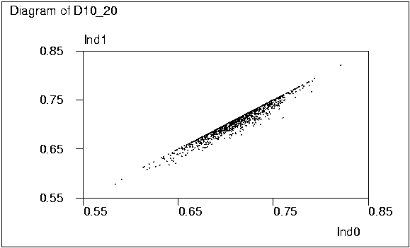
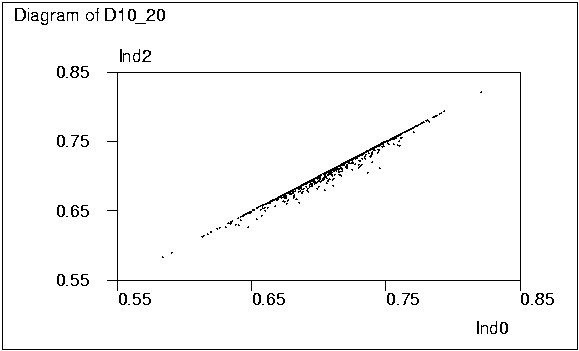
It is interesting to see how closely the two stepwise solutions Ind1 and Ind2 are related to the `true' one Ind0. The two graphs obtained by activating the PLOT commands on lines 73 and 74 tell something about this.

The classified frequencies of ratios Ind1/Ind0 and Ind2/Ind0 given already as a table were calculated as follows:

17 1 SURVO 98 Wed Jul 07 14:48:44 1999 D:\TRE\ 2000 100 0

77 *....................................................................... 78 *VAR R1=Ind1/Ind0 TO D10_20 79 *....................................................................... 80 *VARIABLES=R1 R1=0.8,0.90,0.95,0.99,0.9999999(<1),1.00 81 *TAB D10_20,CUR+1 82 *TABLE D10_201 A,B,F N=1000 83 A R1 * 84 * 0.90 0 85 * 0.95 2 86 * 0.99 335 87 * <1 260 88 B 1.00 403 89 * 90 *....................................................................... 91 *VAR R2=Ind2/Ind0 TO D10_20 92 *....................................................................... 93 *VARIABLES=R2 R2=0.8,0.90,0.95,0.99,0.9999999(<1),1.00 94 *TAB D10_20,CUR+1_ 95 *TABLE D10_201 C,D,F N=1000 96 C R2 * 97 * 0.90 0 98 * 0.95 0 99 * 0.99 81 100 * <1 167 101 D 1.00 752 102 *

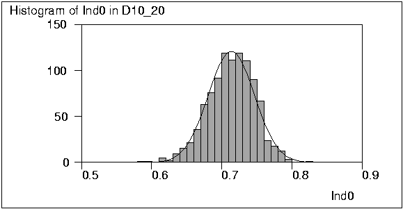
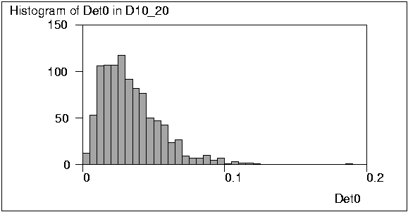
It can also be noted that in this case the distribution of Ind0 is close to normal while that of Det0 is rather skewed as seen from graphs plotted by the HISTO commands of Survo.

18 1 SURVO 98 Thu Jul 08 10:49:38 1999 D:\TRE\ 2000 100 0

102 *....................................................................... 103 *HISTO D10_20,Ind0 / Ind0=0.5(0.01)0.9 FIT=Normal 104 *....................................................................... 105 *HISTO D10_20,Det0_ / Det0=0.0(0.005)0.2 106 *

The solutions were studied also in higher dimensions. One typical example is described below.

6 1 SURVO 98 Thu Jul 08 17:02:09 1999 D:\TRE\ 2000 100 0

1 * 2 *m=15 n=100 3 *C(n,m)=5.3598337040381e+020 (Enormous amount of combinations) 4 *MAT A=ZER(m,n) 5 *MAT #TRANSFORM A BY 0.5-rand(199987) 6 *MAT C=MTM(NRM(A)) 7 * 8 *To measure time elapsed in seconds, 9 *the following 3 commands are executed automatically in succession: 10 *TIME COUNT START 11 *MAT #MAXDET(C,15,S,1) / Original stewise solution 12 *TIME COUNT END 0.600 Time in seconds 13 * 14 *MAT S / *S~maxdet(C)~0.0362487_orthogonality~0.807086 100*1 15 * 16 *TIME COUNT START 17 *MAT #MAXDET(C,15,S,2) / Improved stepwise solution 18 *TIME COUNT END 29.550 19 * 20 *MAT S / *S~maxdet(C)~0.0395331_orthogonality~0.810455 100*1 21 * 22 *....................................................................... 23 *Purely random combinations: 24 *N=10000 Number of random combinations to be studied 25 *RND=19997 Seed of the pseudo random number generator 26 *TIME COUNT START 27 *MAT #MAXDET(C,15,S,3) 28 *TIME COUNT END 9.830 29 * 30 * 31 *MAT S / *S~maxdet(C)~0.000564048_orthogonality~0.670724 100*1 32 * 33 *9.83*C(100,15)/100000= 24903171733704(s:year)=789150.7668522 34 *Thus about 800000 years would be needed for exhaustive search! 35 * 36 *....................................................................... 37 *Random combinations with improvement option: 38 *N=100 RND=199977 39 *TIME COUNT START 40 *MAT #MAXDET(C,15,S,4) 41 *TIME COUNT END 27.570 42 * 43 *MAT S_ / *S~maxdet(C)~0.00130791_orthogonality~0.695115 100*1 44 *

This example indicates that only stepwise solutions are possible in practice. Making of purely random combinations (lines 23-31, option 3 in #MAXDET) does not produce satisfactory results, but gives a basis for estimating the time needed for exhaustive search (lines 33-34).
     Option 4 (lines 37-43) improves each random combination in the same way as option 2 improved the original stepwise selection. It seems to work better than option 3 but is still far away from stepwise alternatives.

Cosine rotation in factor analysis

As mentioned earlier the stepwise algorithm has its roots in a rotation problem of factor analysis. The original idea without explicit algorithm was presented by Yrjö Ahmavaara in a Finnish text book of factor analysis already in 1958 with the name Cosine rotation.
     When making statistical computer programs I talked about this problem with Touko Markkanen and Martti Tienari in 1961 and these discussions led me to the determinant criterion and to the first form of the stepwise algorithm.

In the standard model of factor analysis (see e.g. Harman, 1967) with m variables and r common factors the mxm correlation matrix R is decomposed into the form

(1) R = FphiF^T + psi

where F is the mxr matrix of factor loadings, phi is the rxr correlation matrix of common factors and psi is the mxm diagonal matrix of variances of unique factors. The decomposition is not unique. If F satisfies (1) so does also any

(2) A = F(T^T)^-1

where T is a non-singular rxr `rotation' matrix.

By making suitable assumptions (e.g. multivariate normality of original variables and by setting extra requirements for F), for example, a unique ML estimate for F can be found by an efficient iterative algorithm presented by Jöreskog (1967).
     From such a `primary' solution several derived solutions more pleasant for `interpretation' can be computed by different rotation methods aiming at `simple structure' so that there are lots of `zeros' and a suitable number of `high loadings' in the rotated factor matrix A obtained according to (2).
     In the current form of Cosine rotation we try to reach `simple structure' by selecting the r most orthogonal rows (variables) from F according to the determinant criterion and letting the r rotated factor axes coincide with the vectors of these selected variables.
     If U is the rxr submatrix of F consisting of those r selected rows and all columns, the rotation matrix will then be

     T = U^T[diag(UU^T)]^-1/2

or in Survo notation simply

     MAT T=NRM(U').

Then A will have a structure where for each of the r selected variables there is one high loading on its own factor and zero loadings in all other factors.

In order to demonstrate how Cosine rotation works, a simulation experiment was made as follows. At first a typical F with `simple structure' and m = 100, r = 7 was selected. Also a suitable factor correlation matrix phi was given. Then R was computed according to (1), and a sample of 1000 observations was generated from the multivariate normal distribution N(0,R) by the Survo command MNSIMUL.
     The sample was saved as a Survo data file F100TEST and factor analysis was performed with 7 factors from this data set. At first correlations were estimated by the CORR command, then ML solution with 7 factors was found by the FACTA command, and Cosine rotation was performed by the ROTATE command. Finally the rotated factor matrix A was compared with the original F.
     The following snapshots from the edit field tell the details:

16 1 SURVO 98 Sun Jul 11 14:01:03 1999 D:\TRE\ 1000 100 0

1 *SAVE FA100 / Factor analysis 2 *m=100 r=7 C(m,r)=16007560800 3 * *GLOBAL* 4 *MAT F=ZER(m,r) 5 *MAT RLABELS "X" TO F 6 *MAT CLABELS "F" TO F 7 *MAT #TRANSFORM F BY 1-2*rand(1999) 8 *MAT H2=ZER(m,1) 9 *MAT RLABELS "X" TO H2 10 *MAT #TRANSFORM H2 BY sqrt(0.6*(1-rand(19994)^2)) 11 *MAT F!=DV(H2)*NRM(F')' 12 *MAT TRANSFORM F BY 0.01*int(100*X#+0.5) 13 * 14 *MATRIX D 15 */// Y1 Y2 Y3 Y4 Y5 Y6 Y7 16 *diag 0.80 0.90 0.70 0.75 0.70 0.75 0.85 17 * 18 *MAT SAVE D 19 *MAT D=DV(D) / *D~DV(D) D7*7 20 *MAT CLABELS "F" TO D 21 * 22 *MAT F(12,1)=D(1,*) 23 *MAT F(27,1)=D(2,*) 24 *MAT F(39,1)=D(3,*) 25 *MAT F(64,1)=D(4,*) 26 *MAT F(68,1)=D(5,*) 27 *MAT F(81,1)=D(6,*) 28 *MAT F(90,1)=D(7,*) 29 *MAT NAME F AS F_ 30 *

These MAT commands have produced the original factor matrix F. Most of the rows are purely random. To introduce some kind of simple structure, 7 rows are replaced systematically by vectors Y1, ..., Y7 each of them having one high loading while other loadings are pure zeros. My aim is to show that Cosine rotation is able to detect this structure from simulated data when the sample size is large enough.

Thus the F matrix has the following contents:

23 1 SURVO 98 Sun Jul 11 14:13:29 1999 D:\TRE\ 1000 100 0

30 * 31 *MAT LOAD F,12.12,CUR+1_ 32 *MATRIX F 33 */// F1 F2 F3 F4 F5 F6 F7 34 *X1 -0.27 -0.34 0.47 0.00 -0.16 0.01 0.04 35 *X2 0.06 0.05 -0.20 0.09 0.19 -0.24 0.02 36 *X3 -0.26 0.23 -0.38 -0.32 0.10 -0.26 0.20 37 *X4 0.20 0.32 -0.31 0.06 0.08 -0.16 -0.50 38 *X5 -0.06 0.16 -0.46 -0.36 0.15 -0.23 0.24 39 *X6 0.11 -0.14 -0.24 0.20 0.30 0.30 -0.03 40 *X7 0.05 0.08 0.52 -0.29 -0.01 -0.39 0.28 41 *X8 0.43 0.36 -0.35 -0.04 -0.02 -0.18 0.27 42 *X9 0.17 -0.06 0.21 -0.16 0.14 0.20 0.22 43 *X10 -0.20 -0.07 -0.20 -0.07 0.33 0.51 0.36 44 *X11 0.42 0.03 -0.04 -0.22 0.04 -0.41 -0.03 45 *Y1 0.80 0.00 0.00 0.00 0.00 0.00 0.00 46 *X13 -0.10 -0.39 0.40 -0.24 0.01 0.25 -0.40 47 *X14 0.49 0.20 -0.32 -0.30 -0.22 -0.10 -0.24 48 *X15 -0.11 0.28 0.57 -0.04 -0.14 0.00 0.35 49 *X16 0.00 0.18 -0.08 0.19 0.19 0.17 -0.02 50 *X17 0.16 0.32 -0.16 -0.44 -0.27 -0.35 -0.25 51 *X18 0.19 -0.60 -0.19 0.31 -0.14 0.04 -0.04 52 *X19 -0.42 -0.17 -0.45 -0.27 -0.05 -0.29 0.16 53 *X20 0.12 0.03 0.26 0.44 -0.42 -0.22 -0.31 54 *X21 -0.15 -0.14 0.06 -0.13 0.16 0.10 -0.06 55 *X22 -0.36 -0.19 0.15 0.40 0.09 0.39 -0.30 56 *X23 0.02 -0.25 -0.32 0.08 0.38 -0.10 -0.28 57 *X24 0.27 0.38 -0.22 0.49 -0.16 0.17 -0.19 58 *X25 -0.10 -0.15 0.17 0.02 0.13 0.03 -0.13 59 *X26 -0.20 0.42 0.42 -0.05 0.39 -0.21 -0.01 60 *Y2 0.00 0.90 0.00 0.00 0.00 0.00 0.00 61 *X28 -0.04 -0.05 -0.05 0.02 -0.07 -0.02 -0.06 62 *X29 0.25 -0.06 0.24 0.05 -0.06 0.10 0.13 63 *X30 -0.11 -0.37 -0.35 0.31 -0.26 -0.36 0.16 64 *X31 0.41 0.19 -0.21 -0.27 -0.33 -0.15 -0.29 65 *X32 -0.25 0.17 -0.29 -0.16 -0.48 0.01 -0.27 66 *X33 0.05 0.31 0.45 -0.16 -0.23 -0.47 0.03 67 *X34 0.43 0.16 -0.22 -0.43 -0.06 0.10 -0.07 68 *X35 -0.21 -0.24 -0.22 -0.30 -0.18 0.35 0.26 69 *X36 -0.12 -0.24 -0.33 0.08 0.12 0.57 -0.17 70 *X37 -0.41 0.38 0.47 0.12 0.09 -0.07 0.15 71 *X38 -0.07 -0.22 0.21 0.10 -0.15 -0.17 -0.27 72 *Y3 0.00 0.00 0.70 0.00 0.00 0.00 0.00 73 *X40 -0.31 -0.01 -0.12 0.35 -0.32 -0.22 0.39 74 *X41 0.29 -0.26 -0.17 -0.25 0.01 0.41 0.31 75 *X42 -0.29 -0.11 -0.37 0.07 0.02 0.34 0.25 76 *X43 -0.28 -0.04 0.16 0.29 -0.22 -0.36 -0.02 77 *X44 0.18 -0.28 -0.34 0.37 0.05 -0.05 -0.09 78 *X45 0.12 0.06 -0.30 -0.32 -0.30 -0.38 0.15 79 *X46 -0.30 -0.05 0.19 0.32 -0.26 0.11 0.50 80 *X47 -0.23 0.37 -0.17 -0.28 -0.32 0.04 -0.33 81 *X48 -0.46 0.22 0.01 0.48 -0.17 -0.27 -0.03 82 *X49 0.00 -0.25 0.12 -0.07 -0.27 -0.19 0.23 83 *X50 0.20 0.21 0.23 0.25 0.20 0.01 0.10 84 *X51 0.10 -0.12 0.11 0.02 -0.20 0.26 -0.13 85 *X52 0.06 0.14 0.14 0.32 -0.12 0.18 0.23 86 *X53 -0.40 0.05 -0.40 -0.28 -0.22 0.26 0.10 87 *X54 -0.15 0.23 -0.03 0.02 -0.24 -0.17 0.06 88 *X55 0.24 0.36 0.07 0.15 0.56 -0.01 0.00 89 *X56 0.09 -0.24 0.29 0.32 0.12 -0.35 -0.35 90 *X57 0.31 -0.05 -0.34 -0.12 0.35 0.10 -0.41 91 *X58 -0.19 0.22 0.21 -0.07 0.24 -0.24 0.24 92 *X59 -0.46 0.17 0.36 0.34 -0.14 0.06 -0.09 93 *X60 -0.20 -0.35 -0.01 -0.32 0.35 -0.39 0.26 94 *X61 0.24 -0.40 0.02 0.37 0.07 -0.32 0.28 95 *X62 0.06 -0.45 0.26 -0.36 0.06 -0.01 -0.25 96 *X63 0.10 0.20 -0.28 -0.20 -0.15 0.46 -0.21 97 *Y4 0.00 0.00 0.00 0.75 0.00 0.00 0.00 98 *X65 -0.10 -0.36 0.17 0.37 -0.36 0.19 0.33 99 *X66 -0.20 -0.22 0.45 0.10 -0.14 0.45 -0.27 100 *X67 -0.42 -0.17 0.16 -0.01 0.06 -0.47 -0.14 101 *Y5 0.00 0.00 0.00 0.00 0.70 0.00 0.00 102 *X69 -0.16 -0.25 0.03 0.20 -0.33 0.14 0.06 103 *X70 0.11 -0.34 0.15 -0.32 0.19 0.23 -0.28 104 *X71 0.02 0.00 -0.05 0.38 0.12 -0.27 -0.04 105 *X72 0.11 -0.27 0.12 0.09 0.05 0.30 -0.28 106 *X73 -0.06 -0.25 -0.01 -0.13 0.20 0.10 -0.28 107 *X74 0.19 0.13 0.26 0.07 -0.26 -0.19 0.20 108 *X75 -0.04 -0.39 -0.11 0.35 0.28 -0.06 0.48 109 *X76 -0.33 0.21 0.07 0.46 -0.13 0.24 0.35 110 *X77 -0.34 -0.20 -0.27 -0.35 -0.32 0.19 -0.11 111 *X78 -0.22 0.24 -0.13 -0.23 0.21 -0.22 -0.21 112 *X79 -0.16 0.14 0.01 0.32 -0.25 0.34 0.09 113 *X80 -0.20 0.28 -0.34 0.31 -0.04 -0.16 -0.33 114 *Y6 0.00 0.00 0.00 0.00 0.00 0.75 0.00 115 *X82 0.08 0.17 -0.09 -0.38 -0.36 0.26 -0.37 116 *X83 0.35 0.36 -0.32 0.03 -0.40 0.11 -0.27 117 *X84 0.16 0.17 0.05 -0.14 -0.13 -0.11 -0.18 118 *X85 -0.34 0.18 -0.20 -0.37 -0.40 -0.27 0.13 119 *X86 0.05 -0.12 -0.20 0.28 -0.26 0.32 -0.03 120 *X87 -0.12 0.12 0.14 -0.49 0.31 -0.38 -0.13 121 *X88 -0.02 -0.08 0.15 0.09 -0.17 0.09 -0.19 122 *X89 0.02 0.04 -0.03 0.04 -0.06 0.01 0.00 123 *Y7 0.00 0.00 0.00 0.00 0.00 0.00 0.85 124 *X91 -0.24 0.28 0.17 -0.18 -0.22 -0.41 0.00 125 *X92 0.02 0.03 -0.03 0.04 -0.03 -0.01 -0.02 126 *X93 0.10 0.17 0.21 -0.44 -0.44 -0.19 -0.30 127 *X94 0.31 0.07 0.19 0.34 0.24 -0.06 -0.01 128 *X95 -0.07 -0.32 0.44 0.01 0.39 0.10 0.07 129 *X96 0.28 0.04 0.14 -0.08 0.34 -0.05 0.38 130 *X97 0.39 0.29 -0.09 -0.20 0.37 0.10 0.01 131 *X98 0.21 -0.39 0.38 -0.25 0.33 0.14 0.27 132 *X99 -0.21 -0.02 -0.19 0.29 -0.01 0.23 0.13 133 *X100 0.13 -0.32 0.22 0.03 -0.11 -0.32 -0.45 134 *

Let all the correlations between factors be rho = 0.2. Then the factor correlation matrix phi and the correlation matrix R having the structure (1) are computed as follows:

12 1 SURVO 98 Sun Jul 11 16:53:50 1999 D:\TRE\ 1000 100 0

135 *....................................................................... 136 *rho=0.2 137 *MAT PHI!=IDN(r,r,1-rho)+CON(r,r,rho) 138 *MAT R=F*PHI*F' 139 *MAT PSI!=IDN(m,m)-DIAG(R) 140 *MAT R=R+PSI_ / *R~F*PHI*F'+PSI 100*100 141 *

     In the next display line 143 tells how a sample of 1000 observations from the multivariate distribution N(0,R) is generated by an MNSIMUL command. The second parameter (*) indicates that means and standard deviations of all variables are 0 and 1, respectively. The sample (100 variables and 1000 observations) is saved in a Survo data file F100TEST.
     The sample correlations are computed from this data file and saved as a 100x100 matrix file CORR.M by the CORR command on line 145.
     The maximum likelihood factorization with 7 factors is performed by the FACTA command (line 146) from the correlation matrix CORR.M. The 100x7 factor matrix is saved as a matrix file FACT.M.
     Finally, Cosine rotation is made by the ROTATE command (line 147) and the rotated matrix is saved as AFACT.M and loaded into the edit field (lines 148-178; certain lines are deleted afterwards).
     Line 149 (giving the labels of the columns) is very important. It tells that variables Y1, ..., Y7 - which were supposed to be factor variables - really form the selected, maximally orthogonal basis for the solution. Already this proves that we have found the original structure from a noisy data. Here we have again a situation where alphanumeric labels turn out to be very useful.

22 1 SURVO 98 Sun Jul 11 16:59:46 1999 D:\TRE\ 1000 100 0

142 * 143 *MNSIMUL R,*,F100TEST,1000,0 144 * 145 *CORR F100TEST 146 *FACTA CORR.M,7 147 *ROTATE FACT.M,7,CUR+1_ / METHOD=COS RESULTS=100 148 *Rotated factor matrix AFACT.M=FACT.M*inv(TFACT.M)' 149 * Y4 Y2 Y7 Y6 Y1 Y3 Y5 Sumsqr 150 *X1 -0.051 -0.329 0.093 -0.016 -0.287 0.475 -0.123 0.443 151 *X2 0.117 0.052 0.046 -0.263 0.046 -0.239 0.139 0.166 152 *X3 -0.297 0.244 0.205 -0.234 -0.310 -0.373 0.078 0.486 153 *X4 0.059 0.358 -0.543 -0.153 0.222 -0.314 0.070 0.602 154 *X5 -0.354 0.116 0.222 -0.244 -0.024 -0.470 0.145 0.489 155 *X6 0.248 -0.105 -0.119 0.355 0.134 -0.189 0.271 0.340 156 *X7 -0.325 0.078 0.373 -0.392 0.027 0.455 0.044 0.614 157 *X8 -0.004 0.309 0.248 -0.153 0.494 -0.322 -0.082 0.535 158 *X9 -0.147 -0.016 0.279 0.208 0.146 0.149 0.111 0.199 159 *X10 0.001 -0.029 0.367 0.498 -0.258 -0.209 0.309 0.590 160 *X11 -0.264 -0.018 -0.026 -0.386 0.452 -0.042 0.091 0.434 161 *Y1 0.000 0.000 0.000 0.000 0.791 0.000 0.000 0.626 162 *X13 -0.302 -0.342 -0.409 0.170 -0.053 0.405 0.073 0.576 163 *X14 -0.280 0.141 -0.252 -0.117 0.515 -0.310 -0.230 0.589 164 *... (73 lines deleted in this display) 165 *X88 0.081 -0.124 -0.163 0.063 -0.018 0.146 -0.154 0.098 166 *X89 0.011 0.099 0.063 -0.009 -0.054 -0.029 -0.113 0.030 167 *Y7 0.000 0.000 0.838 0.000 0.000 0.000 0.000 0.703 168 *X91 -0.241 0.275 0.021 -0.401 -0.236 0.118 -0.217 0.412 169 *X92 0.047 0.018 -0.021 -0.001 0.027 -0.034 -0.082 0.012 170 *X93 -0.458 0.133 -0.285 -0.199 0.076 0.167 -0.378 0.525 171 *X94 0.359 0.041 -0.013 -0.030 0.325 0.201 0.213 0.323 172 *X95 0.008 -0.286 0.177 0.066 -0.076 0.405 0.414 0.459 173 *X96 -0.060 0.046 0.395 -0.062 0.315 0.136 0.324 0.389 174 *X97 -0.182 0.258 -0.035 0.093 0.421 -0.063 0.380 0.436 175 *X98 -0.264 -0.367 0.248 0.165 0.242 0.356 0.396 0.636 176 *X99 0.298 -0.043 0.159 0.224 -0.196 -0.163 -0.045 0.233 177 *X100 -0.001 -0.273 -0.455 -0.364 0.125 0.208 -0.093 0.482 178 *Sumsqr 7.224 5.562 6.219 6.081 6.376 6.352 5.982 43.796 179 * 180 *Rotation matrix TFACT.M 181 * Y4 Y2 Y7 Y6 Y1 Y3 Y5 182 *F1 -0.623 -0.462 -0.429 -0.481 -0.615 -0.599 -0.577 183 *F2 -0.472 0.510 -0.306 -0.217 0.425 0.100 0.015 184 *F3 -0.198 0.113 0.666 -0.449 -0.078 -0.001 0.292 185 *F4 0.174 0.530 0.069 -0.052 -0.354 0.357 -0.462 186 *F5 -0.039 -0.411 -0.336 -0.388 -0.127 0.635 0.053 187 *F6 0.514 -0.078 -0.039 -0.586 0.293 -0.235 -0.164 188 *F7 -0.233 -0.241 0.400 0.151 0.455 0.213 -0.581 189 * 190 *Factor correlation matrix RFACT.M 191 * Y4 Y2 Y7 Y6 Y1 Y3 Y5 192 *Y4 1.000 0.149 0.192 0.161 0.186 0.194 0.264 193 *Y2 0.149 1.000 0.198 0.202 0.224 0.223 0.194 194 *Y7 0.192 0.198 1.000 0.184 0.271 0.132 0.162 195 *Y6 0.161 0.202 0.184 1.000 0.203 0.171 0.155 196 *Y1 0.186 0.224 0.271 0.203 1.000 0.231 0.183 197 *Y3 0.194 0.223 0.132 0.171 0.231 1.000 0.131 198 *Y5 0.264 0.194 0.162 0.155 0.183 0.131 1.000 199 *

The ROTATE command has saved the rotation matrix T as TFACT.M and the estimate of factor correlations as RFACT.M. We see that all correlations (lines 190-198) are reasonably close to the theoretical value rho = 0.2.

It remains to be checked how good is the match between the original factor matrix F (saved as matrix file F) and the rotated factor matrix A = AFACT.M obtained from the sample.
     Due to possible ambiguity in rotation it is reasonable to seek an rxr transformation matrix L which minimizes
     f(L) = ||AL - F||₂.
The solution of this least squares problem is
     L = (A^TA)^-1A^TF.
Besides L - especially in connection with factor analysis - it is worthwhile to compute the residual matrix
     E = AL - F
or compare AL and F by other means as done in general situations by Ahmavaara already in 1954. Here we only compute the sum of squares of the elements of E which is the same as the minimum of f(L) squared.

13 1 SURVO 98 Sun Jul 11 17:43:40 1999 D:\TRE\ 1000 100 0

200 *....................................................................... 201 *MAT A=AFACT.M / *A~A 100*7 202 *MAT L=INV(A'*A)*A'*F 203 *MAT LOAD L,12.1234,CUR+1 204 *MATRIX L 205 *INV(A'*A)*A'*F 206 */// F1 F2 F3 F4 F5 F6 F7 207 *Y4 -0.0071 -0.0068 -0.0266 0.9724 0.0549 -0.0136 0.0185 208 *Y2 0.0005 1.0425 0.0003 -0.0263 0.0362 -0.0166 0.0007 209 *Y7 -0.0015 -0.0039 0.0217 -0.0079 0.0323 -0.0060 0.9761 210 *Y6 0.0132 -0.0279 -0.0345 -0.0578 0.0004 1.0244 0.0282 211 *Y1 0.9486 0.0255 -0.0011 -0.0284 -0.0058 0.0130 0.0355 212 *Y3 0.0217 -0.0160 1.0180 0.0632 -0.0444 0.0255 -0.0621 213 *Y5 -0.0198 -0.0187 -0.0164 0.0206 0.9833 -0.0059 -0.0224 214 * 215 * 216 *MAT S=SUM(SUM(A*L-F,2)') 217 *MAT_S(1,1)=0.45053133919049 Residual SS 218 * 219 *MAT S0=SUM(SUM(F,2)') 220 *MAT_S0(1,1)=43.5683 Original SS 221 *

Matrix L is rather accurately a permuted identity matrix as seen on lines 204-213. Thus there is almost a perfect match between the original and estimated factors. The residual sum of squares is fairly small (line 217) and confirms that this form of factor analysis (in this case) has managed to recover the original factor structure.

It should be noted that if the data set F100TEST is centered and normalized by columns (variables) and the most orthogonal submatrix is searched for by the MAT #MAXDET operation (thus applied to CORR.M), none of the Y variables appear among the 7 selected ones:

27 1 SURVO 98 Mon Jul 12 13:13:06 1999 D:\TRE\ 1000 100 0

222 *....................................................................... 223 *MAT #MAXDET(CORR.M,7,S) 224 *MAT FSEL7=SUB(F,S,*) 225 *MAT LOAD FSEL7,12.12,CUR+1_ 226 *MATRIX FSEL7 227 *SUB(F,S,*) 228 */// F1 F2 F3 F4 F5 F6 F7 229 *X1 -0.27 -0.34 0.47 0.00 -0.16 0.01 0.04 230 *X9 0.17 -0.06 0.21 -0.16 0.14 0.20 0.22 231 *X42 -0.29 -0.11 -0.37 0.07 0.02 0.34 0.25 232 *X61 0.24 -0.40 0.02 0.37 0.07 -0.32 0.28 233 *X72 0.11 -0.27 0.12 0.09 0.05 0.30 -0.28 234 *X89 0.02 0.04 -0.03 0.04 -0.06 0.01 0.00 235 *X92 0.02 0.03 -0.03 0.04 -0.03 -0.01 -0.02 236 *

This shows how important it is to purify the data from extra noise caused by unique factors before trying to find a simple structure and this happens by making first the decomposition (1) by ML principle, for example.

It is also interesting to see how many observations are actually needed in this example for detecting the correct structure.
     By a simple sucro similar factor analyses were made for all subsamples of observations 1, 2,..., N for N = 101, 102,..., 1000 and in each case the residual sum of squares, maximum absolute residual, and a dummy variable telling whether the `correct' Y basis was found, were calculated.
     This information was collected in a Survo data file and the following graphs could then be plotted.

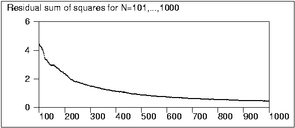
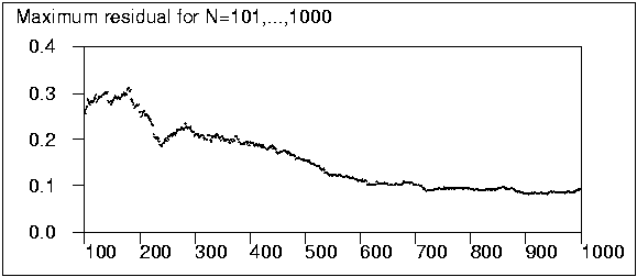
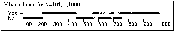
The largest N for which the original basis was not found was 749. Even in this case six of the seven Y variables was selected but Y5 was replaced by X55 which was the variable with highest correlation with Y5. Similar digressions took place also in many other cases, but anyhow when N was above 300 one can say that the original factor structure was decently recovered. At least below 250 both the residual sums of squares and the maximum residuals are so high that finding the original structure often fails.
     To be on the safe side, in this kind of situation at least 600 observations should be available. I think that in too many real applications which I have seen during the past 40 years, the number of observations has been too small or the sample has been too heterogeneous.

For certain, partly justified reasons factor analysis has bad reputation among statisticians. I feel, however, that sometimes the criticism has gone too far or rests on false premises as done by Francis (1974) and quoted by Seber (1985). Some of the erratic conclusions of Francis have been rectified by Mustonen and Vehkalahti (1997).

Structure of the matrix interpreter

SURVO 98 is a collection of hundreds of program modules and other system files. All the modules are working under the control of the Survo Editor which is the visible part of the system (as seen in all previous displays) and this editor calls program modules into use as child processes according to the activations of the user. The user sees Survo as one large program or environment without a need to know about the internal structure of the system.

When a command in the edit field is activated, the Editor recognizes and executes it. Simple commands (like those related to text processing or small-scale calculations) are performed by the editor itself. Other commands (like statistical and graphics commands) are only interpreted to certain extent and then the editor calls a suitable module (i.e. spawns it as a child process) for actual execution. The module obtains all pertinent information from the editor (through a single pointer that points at a table of pointers of Survo's internal workspace) and calculates and produces results to be shown in the edit field and/or in matrix files and other files for the results. After termination of the child process the control returns to the editor with eventual results properly displayed and the user can continue the work.

This architecture enables continuous extension of the system itself even while using it. In fact, all programming and system development related to Survo is done while using Survo. Program modules are written in C according to certain simple rules described in Mustonen (1989) and in www.helsinki.fi/survo/c/index.html. For example, a new module is created by typing the program code in the edit field, then saving it, and compiling it by the Watcom C Compiler with the DOS /32A Extender. As a result we have a new Survo module which immediately can be activated by its name like any other module. The modules are genuine 32-bit programs in protected mode and they have access to all memory up to 2 gigabytes in the CPU.

All commands of the matrix interpreter have MAT as their first `word'. When such a command is activated, the editor calls the matrix interpreter (module _MAT.EXE) which executes most MAT commands directly. Certain additional commands (like MAT #MAXDET) are external to the matrix interpreter. They appear in their own program module(s) and are called in turn by the matrix interpreter (as `grandchildren' of the editor).

The matrix interpreter (as other Survo modules) uses dynamic space allocation for all workspace they need during their use. This space is freed automatically after execution of the command. For example, in matrix multiplication (MAT C=A*B) space is reserved for the operands A and B as well as for the result C just according to their true dimensions. The operands must be located as matrix files (as A.MAT and B.MAT in the example). After they are loaded into the central memory the results are computed and saved as matrix files (C.MAT in the example). Typically only three spaces for matrices are used simultaneously. Thus more complicated commands like computing of a Mahalanobis' distance by

MAT D2=(X-MY)'*INV(S)*(X-MY)

are automatically preprocessed and converted to a series of basic matrix commands. The above MAT command is translated within the matrix interpreter into 4 MAT commands

MAT %%1=X-MY
MAT %%2=INV(S)
MAT %%2=%%2*%%1
MAT D2=%%1'*%%2

where %%1, %%2,... are temporary matrices (matrix files).
     Although a lot of loading and resaving of matrices takes place during matrix computations, no significant loss is encountered in execution times due to proper cache memory settings. On the contrary, it is worthwhile to have all matrices automatically saved in permanent files even if the work is suddenly interrupted for some reason...

Acknowledgements

I am grateful to Simo Puntanen and Kimmo Vehkalahti, who have been helpful in many respects during preparation of this manuscript.

References

Ahmavaara, Y. (1954).

Transformation analysis of factorial data. Ann.Acad.Sci.Fenn., B88,2.

Ahmavaara, Y., and Vahervuo, T. (1958).

Johdatus Faktorianalyysiin, (Introduction to Factor Analysis, In Finnish). WSOY.

Francis, I. (1974).

Factor analysis: fact or fabrication. Math.Chron., 3, 9-44.

Golub, G.H., and Van Loan, C.F. (1989).

Matrix Computations, Second Edition. The Johns Hopkins University Press.

Harman, H.H. (1967).

Modern Factor Analysis, Second Edition. The University of Chicago Press.

Jöreskog, K.G. (1967).

Some contributions to maximum likelihood factor analysis. Psychometrika, 32, 443-482.

Kowal, R.R. (1971).

Disadvantages of the generalized variance as a measure of variability. Biometrics, 27, 213-216.

Mustonen, S. (1963).

SMS, a system of matrix subroutines for use with the 803 autocode, National Elliott computer application program LM21, Elliott Computing Division.

Mustonen, S. (1980).

SURVO 76 EDITOR, a new tool for interactive statistical computing, text and data management, Research Report No. 19. Dept. of Statistics, University of Helsinki.

Mustonen, S. (1982).

Statistical computing based on text editing, Proceedings in Computational Statistics, 353-358, Physica-Verlag, Wien.

Mustonen, S. (1989).

Programming SURVO 84 in C, Dept. of Statistics, University of Helsinki.

www.helsinki.fi/survo/c/index.html

Mustonen, S. (1992).

Survo - An Integrated Environment for Statistical Computing and Related Areas, Survo Systems, Helsinki.

Mustonen, S. (1997).

A measure for total variability in multivariate normal distribution. Computational Statistics & Data Analysis, 23, 321-334.

Mustonen, S., and Vehkalahti, K. (1997).

Survo as an environment for statistical research and teaching. Bulletin of ISI, Istanbul, Proceedings 2, 69-72.

www.helsinki.fi/survo/isi97.html

Seber, G.A.F. (1985).

Multivariate Observations, Wiley.

The website of Survo (www.helsinki.fi/survo/eindex.html) contains more information about the topic of this talk.

This paper has been prepared entirely by using SURVO 98 and it is printed by the PRINT operation of Survo on a PostScript printer. The paper has also been converted into HTML format by Kimmo Vehkalahti by his own HTML driver for the PRINT operation.

• Etusivu / Front page
• Linkit / Links

http://www.helsinki.fi/survo/matrix99.html - 1999-08-05